當多項式混沌跨過折疊點

多項式 surrogate 的吸引力很直接：先花一批較昂貴的模型評估建立近似式，之後便可用廉價代數運算進行大量不確定性傳播、統計量估計或事件判別。當輸入到輸出的關係平滑，這種做法往往相當有效；但若模型響應不只是彎曲，而是在 saddle-node fold 附近由一條穩定分支跳到另一條穩定分支，一個連續的全域多項式便要同時代表兩段平滑曲線及中間的不連續跳躍。它可能在跳點附近振盪、移動門檻交點，甚至把機率質量放到物理響應範圍之外。

本專案用一個刻意簡化、完全合成、無因次的 non-isothermal continuous stirred-tank reactor（CSTR）檢查這個問題。不確定的 Damköhler number 以解析 ignition fold 為中心。全域方法用 16 個 Gauss–Legendre 節點建立 degree-15 Legendre surrogate；局部方法把輸入區間在已知 fold 處一分為二，每邊以 8 個節點建立 degree-7 surrogate。兩者用於 fit 的 forward evaluation 都剛好是 16 次。

然而，局部方法事先得到解析 fold 位置。這個 fold 是一個 analytic oracle，其推導、尋找或設定成本沒有計入 16 對 16 的 fit budget。因此本文只稱它為 fold-aligned，絕不稱為 adaptive。這不是 total-cost comparison，也沒有證明自動演算法能從 16 次評估找出分界，更沒有物理、工業安全或普遍優越性的結論。

在這個範圍內，第一階段結果很明確。全域 surrogate 的 response RMSE 是 $0.0783280594$ ，fold-aligned surrogate 是 $0.000248551855$ ，相差約 $315.14$ 倍；Wasserstein-1 error 分別為 $0.0439521168$ 與 $5.03489790\times10^{-5}$ ，相差約 $872.95$ 倍。在已申明的 cold-start、quasi-static、increasing- $Da$ 、right-continuous history 下，解析 hot-state probability 是 $0.5$ ；全域結果為 $0.4710647474$ ，fold-aligned 結果為 $0.5$ 。全域 surrogate 還產生 $0.0531311035$ 的 invalid-support mass，局部版本在既定 evaluation grid 上則為零。

這些數值只屬於單一固定的第一階段 benchmark，不是新 multi-element PCE 方法的發明。文獻審查把研究結論定為 REFRAME，因為 polynomial chaos、分岔不確定性、random-space partition、automatic discontinuity detection 與 uncertain CSTR 都有直接先行研究。這個標記指比較一個精確的 matched-fit 問題，而不是宣稱發明 multi-element polynomial chaos。

折疊點附近發生了甚麼

問題	結果	為何重要
使用了甚麼模型？	合成、無因次 CSTR	它是 canonical numerical model，不是經實驗校準的反應器。
如何定義 branch history？	cold start、準靜態增加 $Da$ 、ignition 處右連續	這是一種固定歷史下的響應，不是有限升溫速率模擬。
使用了甚麼不確定性？	$Da=Da_{\mathrm{ign}}+0.008\xi$ ， $\xi\sim U[-1,1]$	輸入分佈對稱並以 ignition fold 為中心。
全域方法如何分配 16 次 calls？	在整個區間建立一個 degree-15 fit	連續 polynomial 必須跨越響應跳躍。
局部方法如何分配 16 次 calls？	兩個 degree-7 fits，每側 8 次	Oracle split 令每個 polynomial 只近似一條 smooth branch。
比較建立了甚麼？	16 項科學檢查全部通過，狀態 SUPPORTED	結果支持這個 smoke comparison，不是普遍方法排名。
哪項成本沒有計入？	解析 fold location	Fit-call budget 相同，但 total setup cost 未比較。

「同一 budget」若沒有說明 budget 的單位，便很容易造成誤解。本研究匹配的是建立 surrogate 所用的 response-model calls。全域方法不需要已知分界，局部方法卻得到精確 fold。若在複雜模型中要靠 continuation、額外 solver calls、pilot samples、classifier 或人工判讀找出 fold，這些都應計入 end-to-end cost。本階段沒有估算這部分，所以不能把「16 對 16」改寫成「相同總成本」。

文獻為何改變了研究問題

專案最初容易形成一個過大的故事：adaptive multi-element polynomial chaos 能在 thermal bistability 下勝過 global PCE。正式運算前的文獻審查顯示，這種說法把已建立的領域當成空白。

Wan 與 Karniadakis 在 2005 年已提出 adaptive multi-element generalized polynomial chaos，核心思想正是當全域 spectral regularity 失效時，在 random space 進行分區（DOI）。Venturi、Wan 與 Karniadakis 在 2010 年把 stochastic bifurcation analysis 用於 Rayleigh–Bénard convection（DOI）。Kuehn 與 Lux 從 random ODE 與 dynamical systems 角度系統處理 bifurcation uncertainty（DOI）。

與本題更直接的工作也已出現。Dréau、Magnain 與 Batailly 研究以 automatic discontinuity detection 建立 multi-element polynomial chaos（DOI）。Kuehn、Piazzola 與 Ullmann 研究帶 random coefficients 的 Allen–Cahn bifurcation uncertainty（DOI）。Gonnella、Khamlich、Pichi 與 Rozza 在 2026 年處理 nonlinear bifurcating problems 的 stochastic perturbation（DOI）；Venier、Gonnella、Pichi 與 Rozza 則討論 polynomial-chaos branch approximation 的 consistency 與 convergence（arXiv DOI）。

兩條鄰近文獻線同樣限制 novelty。Bourgey、Gobet 與 Rey 比較 indicator functions 的 polynomial-type chaos expansions；當 surrogate 最後要用來計算超標機率時，這類結果非常相關（DOI）。CSTR uncertainty 亦非未開發領域：Ratto 與 Paladino 在 2000 年分析 controlled CSTR 的 fluctuating 與 uncertain parameters（DOI）；Du、Budman 與 Duever 其後把 PCE-based Markov models 用於 probabilistic robust self-tuning control（DOI）。

這十篇 primary works 足以確立幾項「既有知識」：全域多項式在非平滑響應上可能失去 spectral efficiency；random-space decomposition 與 ME-PCE 已建立；adaptive 或 automatic discontinuity localization 已有人研究；polynomial chaos 已與 bifurcation analysis 結合；uncertain CSTR 也已有機率方法。本文不能把任何一點寫成自己的發現。

因此，重新框定後的研究問題是：

在一個固定、以 ignition fold 為中心的輸入分佈，以及一個明確申報的 branch history 下，若兩種 surrogate 各使用 16 次 fit evaluation，全域 degree-15 polynomial 與 oracle fold-aligned degree-7+7 polynomial 的可靠性有何差別？

這個問題仍有價值，因為每個容易偷換的條件都被放在明面：branch selection、事件門檻、fit budget、oracle 資訊、reference construction 與 decision rule。文獻搜索支持「縮窄問題」的判斷，但不等於證明世界上沒有任何相似 benchmark；本地 smoke result 也不會推翻已建立的理論或方法。

模型：一個可解析處理的 canonical CSTR

模型狀態是無因次 reactant concentration $c$ 與 temperature rise $\theta$ 。activation parameter 為 $a$ ，heat-release parameter 為 $B$ ，Damköhler number 為 $Da$ ：

\frac{dc}{dt} =1-c-Da\,c\exp\!\left(\frac{a\theta}{a+\theta}\right),

\frac{d\theta}{dt} =-\theta+B\,Da\,c\exp\!\left(\frac{a\theta}{a+\theta}\right).

第一階段固定 $a=20$ 、 $B=8$ 。這兩個值只定義合成 benchmark；沒有對應某種化學反應、反應器體積、冷卻能力、停留時間、進料濃度或工業操作區間。

穩態時，把第一式乘 $B$ 再與第二式相加，nonlinear reaction term 正好消去：

B(1-c)-\theta=0.

所以所有正穩態都滿足

c=1-\frac{\theta}{B}.

代回穩態式，便可用 $\theta$ 精確參數化 equilibrium curve：

Da(\theta) =\frac{\theta}{B-\theta} \exp\!\left(-\frac{a\theta}{a+\theta}\right), \qquad 0<\theta<B.

上式兩部分是相乘，即

Da(\theta) =\frac{\theta}{B-\theta} \;\times\; \exp\!\left(-\frac{a\theta}{a+\theta}\right).

程式實作的明確形式是 $\frac{\theta}{B-\theta}\exp(-a\theta/(a+\theta))$ 。利用這條 exact scalar curve，benchmark 不需要靠 time integration 猜測穩態，也不受步長或 transient stopping rule 影響。

解析推導兩個 folds

Fold 是 $Da(\theta)$ 的 stationary point。對其 logarithm 微分較簡潔：

\frac{d}{d\theta}\log Da(\theta) =\frac{1}{\theta} +\frac{1}{B-\theta} -\frac{a^2}{(a+\theta)^2}.

令它為零並清除分母，得到 quadratic：

(a^2+B)\theta^2 +aB(2-a)\theta +Ba^2=0.

在 $a=20$ 、 $B=8$ 時， $(0,B)$ 內有兩個 roots。較低溫的 turning point 是 ignition fold：

\theta_{\mathrm{ign}}=1.3814801666464074,\qquad Da_{\mathrm{ign}}=0.057329640075221795.

較高溫的 turning point 是 extinction fold：

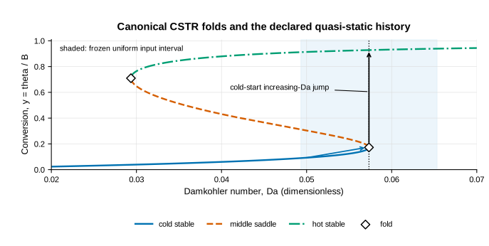
\theta_{\mathrm{ext}}=5.677343362765358,\qquad Da_{\mathrm{ext}}=0.029354991549934553.

雖然 ignition 的 $\theta$ 較低，其 $Da$ 卻較高；這個次序正是 S-shaped curve 的來源。在 $Da_{\mathrm{ext}}$ 與 $Da_{\mathrm{ign}}$ 之間，有 stable cold、unstable middle saddle 與 stable hot 三個 equilibria。程式用 Jacobian eigenvalues 核對 stability，而不是僅按溫度高低貼標籤。

解析結果另由獨立 scan 找 logarithmic derivative 的 sign changes，再以 bisection 求根。Ignition 的解析與數值 $Da$ 差 $6.94\times10^{-18}$ ，extinction 差 $0$ ；兩個 $\theta$ 差分別為 $9.44\times10^{-14}$ 及 $2.30\times10^{-13}$ 。Fold derivative residual 分別為 $2.22\times10^{-16}$ 及 $0$ ，finite-difference second derivative 亦非零，符合 frozen tolerance 下「兩個 simple folds」的要求。

無因次 CSTR 平衡曲線，標出穩定冷分支、穩定熱分支、中間 saddle、ignition 與 extinction folds、不確定輸入區間及 cold-start 跳躍。 — Canonical equilibrium curve 與已申明 branch history；這是右連續的準靜態 history operator，不是有限 ramp rate 的 ignition simulation。

沒有 history，就沒有唯一 response

在 bistable interval 內，同一 $Da$ 可同時有 cold 與 hot 兩個 stable equilibria。若只叫 nonlinear root solver 回傳「一個 equilibrium」，答案會依初值、求解器 basin 或 continuation direction 而變。因此 branch history 不是事後解釋，而是 response definition 的一部分。

第一階段固定以下規則：

從 $Da_0=0.020$ 開始；
準靜態、單調增加 $Da$ ；
當 $Da<Da_{\mathrm{ign}}$ 時沿 stable cold branch；
到達 ignition fold 時轉到 hot branch，並採 right-continuous convention。

$Da_0=0.020$ 低於 extinction value $0.02935499155$ 。Branch enumeration 在該點只找到一個 equilibrium，而且它是 stable cold state。這項檢查防止起始分支歧義被悄悄帶入結果。

定義 conversion-like response

y(Da)=\frac{\theta(Da)}{B}.

按上述 history，

y(Da)= \begin{cases} \theta_{\mathrm{cold}}(Da)/B, & Da<Da_{\mathrm{ign}},\\ \theta_{\mathrm{hot}}(Da)/B, & Da\ge Da_{\mathrm{ign}}. \end{cases}

Cold branch 在 fold 的左極限是 $0.1726850208$ ，右連續 hot value 是 $0.9279002591$ 。兩者之間的大跳躍不是 numerical noise，而是已申明 history operator 在 bistable diagram 上的選擇。

此處沒有模擬有限速度增加 $Da$ ，沒有 dynamic bifurcation delay，沒有 thermal noise，也沒有隨機 branch occupancy。因此下文的 hot probability 是「輸入不確定性經指定 history 映射後」的機率，不是 steady-state occupancy probability，更不是物理反應器的事故機率。

以 fold 為中心的不確定性

輸入固定為

\xi\sim U[-1,1],\qquad Da=Da_{\mathrm{ign}}+0.008\xi.

所以實際 $Da$ interval 是

[0.049329640075221795,\;0.0653296400752218],

而 ignition fold 恰好位於 $\xi=0$ 。定義 $y\ge0.8$ 為 hot。在已申明 response 中， $\xi<0$ 屬 cold side， $\xi\ge0$ 由 right-continuous rule 進入 hot side，而且 hot value 高於 $0.8$ 。由 uniform symmetry，

\Pr(y\ge0.8)=\Pr(\xi\ge0)=0.5.

這個 $0.5$ 並不是艱難的 rare-event calculation。它提供一項透明的 event check：如果 surrogate 把 jump 拉平或把 threshold crossing 移位，event probability 便會立刻反映。

全域 degree-15 Legendre surrogate

因為 $\xi$ 在 $[-1,1]$ uniform，Legendre basis 是自然選擇。全域近似為

\widehat y_G(\xi)=\sum_{k=0}^{15}\alpha_kP_k(\xi).

16 個 Gauss–Legendre nodes 提供 16 次 response evaluation，並用 quadrature projection 得到 degree-15 coefficients。程式核對 Gauss weights sum to two、discrete Legendre orthogonality，以及 collocation-node reconstruction。全域最大 node reconstruction error 只有 $5.995\times10^{-15}$ 。

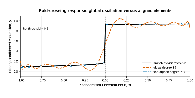
這項結果很關鍵：全域 surrogate 的問題不是明顯的 linear algebra bug，也不是節點資料沒有重建。它正確擬合自己看到的 nodes，但 continuous polynomial 必須跨越 discontinuous response，因此代表能力才是瓶頸。它在 jump 附近產生 oscillation，並把 $y=0.8$ 的 surrogate crossing 移至 $Da=0.05779260412$ ，較真實 transition 高約 $4.63\times10^{-4}$ 。對 uniform input 而言，這個 shift 會直接變成 probability bias。

Oracle fold-aligned degree-7+7 surrogate

局部方法用已知解析 ignition fold 把 interval 分成

I_-=[Da_{\mathrm{ign}}-0.008,\;Da_{\mathrm{ign}}], \qquad I_+=[Da_{\mathrm{ign}},\;Da_{\mathrm{ign}}+0.008].

每個 element 各用 8 個 Gauss–Legendre evaluations 建立 degree-7 expansion：

\widehat y_{\mathrm{FA}}(Da)= \begin{cases} \sum_{k=0}^{7}\beta^-_kP_k(\eta_-(Da)), & Da<Da_{\mathrm{ign}},\\ \sum_{k=0}^{7}\beta^+_kP_k(\eta_+(Da)), & Da\ge Da_{\mathrm{ign}}. \end{cases}

$\eta_-$ 與 $\eta_+$ 分別把兩個 physical elements 映到 $[-1,1]$ 。每個 polynomial 只需近似一條 smooth branch，而 discontinuity 由 element boundary 承擔。左、右 collocation-node reconstruction errors 分別為 $1.055\times10^{-15}$ 及 $6.328\times10^{-15}$ ，總評估數 $8+8=16$ 。

但 split 並非從 16 個 values 自動發現。它由 analytic fold oracle 預先提供。因此不能稱為 adaptive，也不能稱為 equal total cost。這個設計回答的是「知道 fold 有多少價值」，而不是「自動找到 fold 需要多少成本」。

跨越 ignition fold 的 branch-explicit conversion reference，對照全域 degree-15 Legendre surrogate 與 oracle fold-aligned 兩個 degree-7 surrogate。 — 兩個 fits 各使用 16 次 forward evaluations；全域多項式在 jump 附近振盪，oracle-aligned elements 分別停留在平滑分支，而 fold discovery cost 未計入。

Reference 如何與 surrogate 分離

Reference response 不使用兩個 surrogate 之一。對每個 evaluation input，都在 exact scalar steady curve 上按指定 branch 進行 deterministic bisection。Cold root 的 bracket 位於 ignition temperature 以下；middle root 位於兩個 fold temperatures 之間；hot root 位於 extinction temperature 以上。這種 branch-explicit 求解可避免 Newton method 因初值而落到錯誤 equilibrium。

Fine reference 用 32,768 個 midpoint cells，coarse check 用 16,384。由 coarse 到 fine，全域 RMSE 只改變 $9.49\times10^{-9}$ ，全域 Wasserstein-1 改變 $1.56\times10^{-9}$ ；fold-aligned 的相應變化為 $8.02\times10^{-8}$ 與 $2.65\times10^{-9}$ 。全部低於預先固定的 $10^{-6}$ reference-grid tolerance。

在 sampled outer branches 中，最大的 real eigenvalue 是 $-0.0026092$ ，仍為負。代表 middle branch 的 Jacobian determinant 是 $-0.6880$ ，符合 saddle；saved maximum steady-state residual 為 $1.294\times10^{-11}$ ，低於 $10^{-10}$ gate。這些 checks 驗證數學分支與 numerical reference，並不驗證某個實際反應器。

Matched-fit result：四組互補指標

完整核心結果如下：

Metric	Global degree 15	Fold-aligned degree 7+7
Fit forward evaluations	16	16
RMSE	$0.0783280594$	$0.000248551855$
Wasserstein-1 error	$0.0439521168$	$5.03489790\times10^{-5}$
Saved absolute mean error	$0.000230612371$	$8.60410194\times10^{-6}$
Hot-state probability	$0.4710647474$	$0.5$
Hot probability absolute error	$0.0289352526$	$0$
Branch classification error rate	$0.0289306641$	$0$
Invalid-support mass	$0.0531311035$	$0$
One-sided fold maximum error	$0.389895981$	$0.00803041325$

RMSE improvement factor 是

\frac{0.0783280594}{0.000248551855}=315.1376975,

Wasserstein improvement factor 是

\frac{0.0439521168}{5.03489790\times10^{-5}}=872.9495157.

這兩個大倍率有清楚的結構原因：local method 得到 global method 沒有的 jump location。合適結論應是「在已知解析 fold 作 element boundary 且 fit call 數同為 16 的條件下，fold-aligned representation 在本案例明顯較準」。它不能被改寫成「ME-PCE 永遠好 315 倍」，也不能被換算成「總成本便宜 315 倍」。

在標準化輸入零點附近，以 logarithmic scale 比較 global 與 fold-aligned surrogate 的 pointwise absolute response error，並標出解析 ignition fold。 — Pointwise comparison 把依賴 grid spacing 的 maximum error 與穩定 one-sided fold-limit diagnostic 分開，並申報零誤差在圖上的 display floor。

為何不能只看一個 average error

Discontinuity 會把很大的 pointwise error 集中在窄區域，RMSE 平方後對這些 errors 非常敏感。另一個平均量實際計算的是 predicted sample mean 與 reference sample mean 之差的絕對值，而不是逐點 absolute error 的平均；正負 oscillations 可先互相抵銷。因此本文稱它為 absolute mean difference，不把 $2.306\times10^{-4}$ 誤寫成一般 MAE，也不以它推論 event reliability 良好。全域 threshold shift 仍造成 $0.02894$ absolute probability error，另有 $5.31\%$ input mass 被映到 invalid response support。

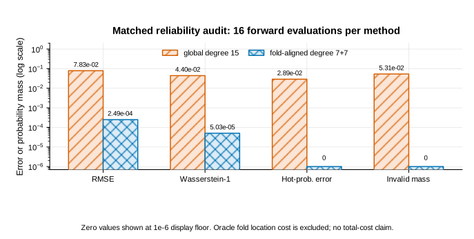
因此 benchmark 同時看四類量：RMSE 衡量 response fidelity；Wasserstein-1 衡量 output distribution；hot probability 檢查明確事件；invalid-support mass 檢查 surrogate 是否創造不可能的 conversion。只有一個漂亮的平均誤差，很容易掩蓋對決策最重要的 failure mode。

為何不採用 dense-grid maximum 作判準

Response 在 fold 右連續且不連續。Dense grid 通常靠近 jump，卻不一定正好取到 jump。Maximum error 會隨「最近 sample 離 jump 多遠」而變；增加 grid density 甚至可能令 maximum 變大，而 surrogate 本身完全沒變。

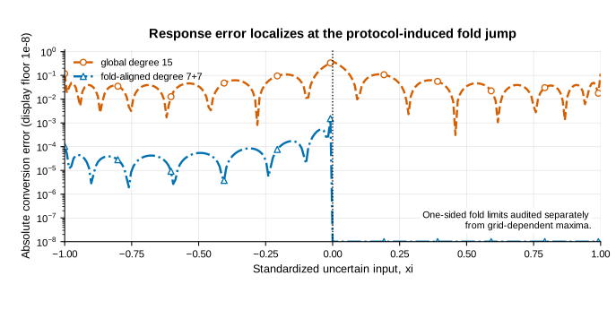
因此 frozen decision rule 沒有把 dense-grid max error 當 pass/fail gate。Result 仍保存它：global 為 $0.389750045$ ，fold-aligned 為 $0.00747760805$ ；但 one-sided fold maximum 才是較穩定 diagnostic。這是 metric design 尊重數學結構的例子，而不是選擇對某方法最有利的數字。

Event probability 與 valid support

解析 history-conditioned hot probability 是 $0.5$ 。全域 polynomial 的 $y=0.8$ crossing 太遲，得到 $0.4710647474$ 。Fold-aligned representation 在 split 使用右側 element，threshold calculation 得到 $0.5$ 。

全域 polynomial 亦會 overshoot $[0,1]$ conversion range；evaluation grid 上對應 input mass 為 $0.0531311035$ 。Fold-aligned measured invalid-support mass 為零。這個零只屬於既定 interval、degree、nodes 與 evaluation；它不是 local polynomial 自動 preserve support 的 theorem。

成對 hatch bars 比較全域與 fold-aligned surrogate 的 RMSE、Wasserstein-1 error、hot-state probability error 及 invalid-support mass，兩者各用 16 次 fit evaluations。 — Fold-aligned surrogate 通過 frozen reliability gates；零值以申報的 display floor 顯示，而 analytic fold-location cost 被排除，所以不能解讀為 total-cost result。

如何判定這次比較

以下 thresholds 在解讀結果前已經固定：

RMSE reduction 至少 $10\times$ ；
Wasserstein-1 reduction 至少 $5\times$ ；
fold-aligned hot-probability error 不超過 $0.01$ ；
evaluation grid 上 fold-aligned invalid-support mass 等於零；
reference、residual、quadrature、reconstruction、fold 與 stability calculations 全部在已申明 tolerance 內。

實際 $315.14$ 與 $872.95$ 超過首兩個 thresholds；hot-probability error 與 invalid-support mass 都為零，其餘 supporting calculations 亦保持在已申明 tolerance 內。因此這個 fold-centered CSTR smoke benchmark 符合所有事前申明的判準。

這些判準只屬於本次比較，不會把 matched-fit result 變成 total-cost result，也不代表所有 ME-PCE。

為何數值結果可信

Analytic fold locations 與 independent scan/bisection 一致，derivative residuals 在 tolerance 內，兩個 folds 亦都是 simple。Frozen initial state 位於 unique stable cold equilibrium；sampled outer branches 保持 stable，middle branch 是 saddle，steady-state residuals 亦在 tolerance 內。這些結果共同支持用來定義 discontinuous response 的 branch history。

兩種 surrogate construction 另有獨立數值核對。Gauss weights 與 discrete Legendre orthogonality 符合預期，collocation nodes 可重建至 roundoff；reference-grid refinement 令各項 error 改變少於 $10^{-6}$ ，而兩個 fits 都使用 16 次 forward evaluations。完整計算重做後，scientific metrics 保持相同。這些吻合支持有限比較，但不會把 oracle-aligned benchmark 變成 automatic 或 total-cost result。

如何測試 split location 的誤差

目前 local surrogate 的優勢包含一項明確資訊：element boundary 恰好等於解析 ignition fold。這項 oracle information 可以用一個直接的 sensitivity experiment 拆開。保持 16 次 fit calls、polynomial degree、input law 及 branch history 不變，只把 split 依序移到 $Da_{\mathrm{ign}}\pm\delta$ 。每個 $\delta$ 都重新計算 response RMSE、Wasserstein-1、hot probability 及 invalid-support mass，便可觀察 localization error 如何傳入四種結果。

對均勻分佈而言，最初的 event-probability penalty 應約為 $|\delta|/0.016$ ，因為 $0.016$ 是整個 input interval 寬度。這條線只是第一階近似。當 misplaced boundary 令其中一個 polynomial 必須跨越部分 jump，ordinary approximation error 會加入，實際曲線便可能離開線性關係。正負位移亦未必完全對稱，因為 cold 與 hot branches 的 curvature 不同。

這個實驗能回答「準確知道 fold 有多重要」，但仍不等於 automatic detection。真正 adaptive comparison 還要加入 pilot calls、continuation、partition decision、定位失敗及 fallback 的成本。Sensitivity study 先量度位置誤差的科學後果，之後才有基礎判斷一個 detector 需要達到多高精度。

為免位置敏感度又受事後選點影響， $\delta$ 網格應在查看結果前固定。Pilot offsets 只用來選擇合理範圍，另留正、負兩側的 held-out offsets 作最終評估；每一點同時報 signed probability shift、RMSE、Wasserstein error、invalid-support mass，並標記移位後的 split 是否跨過 collocation node。這樣才可把 locator bias 與普通 polynomial-fit error 分開，而不是只以一條平均曲線掩蓋方向差異。

Split 偏向 cold side 與偏向 hot side 亦應分開報告。若 boundary 放在真實 fold 左側，右側 polynomial 的 element 會包含一小段 cold response，然後才跨入 hot branch；若 boundary 放在右側，左側 polynomial 會被迫包含 jump 之後的一小段 hot response。兩種情況都令其中一個本來 smooth 的 element 重新遇到 discontinuity，但受影響的 branch、node placement 與 curvature 不同。只畫 $|\delta|$ 的平均曲線可能會掩蓋這個方向差異。

每個 misplaced-split case 應保留與目前相同的四類量，而不是只看 RMSE。即使整體 response error 仍小，threshold crossing 也可能移動；即使 hot probability 尚算接近，polynomial 仍可能在 $[0,1]$ 以外產生 invalid-support mass。Wasserstein-1 則檢查 output distribution 是否因局部 oscillation 而改形。四個量一起讀，才能分辨「事件邊界稍為移位」與「整個 surrogate representation 已重新跨越 jump」。

這項 sensitivity test 也有清楚的反證結果。若很小的 localization error 已把 $315.14$ 與 $872.95$ 的優勢大幅消除，便表示 oracle 結果對 split precision 極敏感，後續方法必須把定位不確定性當成主要誤差來源。若優勢在一段可量度的 $\delta$ 範圍內仍保留，才有理由進一步研究 detector 能否以合理成本達到該範圍。兩種答案都比直接宣稱 local method 普遍較好更有用。

正負 $\delta$ 的結果亦應分開畫出，讓讀者直接看到 branch curvature 與 node allocation 是否造成不對稱，而不是用單一平均值把方向效應消去。

限制不是附註，而是結論的一部分

第一，fold knowledge 是 privileged information。局部 fit 前已提供 exact analytic split，且 setup cost excluded。真正 adaptive algorithm 必須偵測 regularity loss、決定是否分區、分配 samples，甚至反覆修訂 partition；這些步驟完全未實作。

第二，equal fit calls 不等於 equal total cost。Canonical scalar curve 可解析推導，令 fold 在此案例很便宜；large-scale simulator 可能要 continuation、adjoint、additional solves 或人工診斷。未來 total-cost benchmark 必須計入 pilot、fold-location、failed searches 與所有正式 calls。

第三，只有一組 order 與 budget：global degree 15 對 local degree 7+7，都是 16 calls。這不能描述 order convergence，不能說明 global method 增加多少節點後足夠，也沒有測試 misplaced split 對 local method 的破壞程度。

第四，input law 對稱且以 fold 為中心，所以 analytic event probability 剛好是 $0.5$ 。Off-center、skewed、correlated、multi-parameter 或 nonuniform uncertainty 都可能改變結果；這些 sweeps 尚未執行。

第五，branch history 是理想化 quasi-static operator。Finite-rate dynamics 可能有 bifurcation delay 與 transient dependence；stochastic system 可能在 deterministic fold 之前切換。本文沒有這些機理。

第六，模型 synthetic 且 dimensionless。沒有 experimental calibration、parameter identification、heat-transfer design、materials constraint、controller validation、hazard analysis 或 chemical safety case。Hot 只表示數學門檻 $y\ge0.8$ 。

第七，zero invalid-support mass 是固定 evaluation construction 的 empirical result，不是 positivity certificate；exact $0.5$ match 也不是 general event-accuracy theorem。單一 discontinuity 的大 improvement factors 不構成 universal superiority。

第八，文獻審查不是「已證明沒有任何相似工作」。它支持保守解讀，不能單獨證明 novelty。

從 threshold shift 直接讀出 probability error

本案例有一個很有教育價值的關係：全域 surrogate 的 event error 並非難以追蹤的黑箱數字，而可由 threshold location 直接核對。真實 right-continuous transition 在

Da_{\mathrm{ign}}=0.057329640075221795,

全域 polynomial 的 $y=0.8$ crossing 卻在

Da_G=0.0577926041163755.

兩者相差

\Delta Da=Da_G-Da_{\mathrm{ign}} =0.0004629640411537.

整個 uniform interval 寬度是 $0.016$ 。若 surrogate 把 hot region 的左界向右移 $\Delta Da$ ，失去的 input probability mass 正好是

\frac{\Delta Da}{0.016} =0.0289352525721.

這與 saved global hot-probability absolute error $0.028935252572106385$ 一致。因此 $0.4710647474$ 不是任意 numerical integration artifact；它等於 $0.5-0.0289352526$ ，可由已保存 threshold root 獨立理解。這也說明即使 response error 只集中在 fold 附近，對 threshold event 的影響仍可直接累積成數個 percentage points。

Fold-aligned surrogate 沒有需要跨過 jump 的單一 polynomial。Event boundary 已由 element boundary 承擔，而 right-continuous rule 把 fold 點交給右側 hot element，所以 threshold probability 回到 $0.5$ 。但這個 exact match 主要反映 oracle alignment 與對稱 input law；若 split 有位置誤差 $\delta$ ，最直接的 probability penalty 便約為 $|\delta|/0.016$ ，直到其他 polynomial crossing errors 介入。這個簡單比例正是未來「misplaced split sensitivity」值得預先註冊的原因。

Branch classification error rate 亦提供交叉檢查。Global value $0.0289306641$ 與 probability error 非常接近，但不完全相同，因為前者在固定 midpoint evaluation grid 上計數，後者由 polynomial threshold roots 作連續 probability calculation。兩者接近支持共同機理；細微差異則提醒我們 grid statistic 與解析 root integration 不應混成同一個量。Fold-aligned 兩者都為零，只代表固定 evaluation resolution 與既定算法。

16 次 evaluation 究竟買到了甚麼

全域 GL16 把全部 16 個 nodes 放在整段 input interval，對應一個 degree-15 expansion。Fold-aligned GL8+GL8 把八個 nodes 放在 cold interval，另八個放在 hot interval，對應兩個 degree-7 expansions。兩者的 coefficient 數都是 16，response calls 也是 16，但 approximation spaces 不同：前者強制整段連續，後者容許 element boundary 上有 jump。

Gauss–Legendre nodes 不包含 interval endpoints。這代表 local fits 並非靠直接在 fold 上取兩個互相矛盾的 values；它們分別從各自 element 內部的 smooth branch samples 建立 one-sided approximations。Right-continuous convention 再決定當輸入剛好等於 split 時使用右側 polynomial。這個細節把數值表示、branch history 與 event convention 串在一起，也解釋為何文章必須明確申報 fold 點屬於哪一邊。

Matched node count 可排除一個簡單混淆：局部結果不是因為偷偷使用更多 response calls。但它不能排除 information advantage。知道 split location 相當於先得到一項對近似空間非常重要的 model structure。公平的 Phase-1 問題是「在同樣 fit calls 下，這項 oracle information 的效果有多大」；公平的後續問題才是「取得及驗證這項 information 要付多少代價」。

未來 total-cost comparison 至少應分開記錄四類開支。第一類是正式 surrogate fit calls；第二類是尋找或追蹤 fold 的 pilot 與 continuation calls；第三類是 partition decision、error indicator 與可能的 repartition calls；第四類是失敗嘗試、solver recovery 與 validation calls。若只報第一類，adaptive method 可能看起來不合理地便宜；若把 analytic derivation 當成免費常識，亦會把 canonical model 的特殊便利錯當成通用能力。

還要區分一次性 setup 與重複使用成本。若同一 fold map 可服務數千次 downstream queries，setup cost 或可攤薄；若 parameters、geometry 或 operating protocol 每次改變都要重新定位 fold，它便不能忽略。兩種情況沒有哪一種可由本 smoke benchmark 決定。未來報告應同時列出一次 fit 的 marginal cost、包含定位的 first-run cost，以及在明確 reuse count 下的 amortized cost，而不是只給一個沒有分母的 speedup。如此才可判斷 oracle advantage 在實際工作流中是否仍有意義。

成本表亦應保存「沒有成功定位 fold」的情況；若只統計成功 runs，automatic method 的可靠性會被高估。對每個 protocol，應預先定義定位失敗如何處理、是否容許 fallback global fit、fallback 的 calls 如何入帳，以及最後 event interval 是否仍有效。這些都是 Phase 1 尚未回答、但在宣稱 deployable workflow 前不可略過的問題。

四張圖各回答不同問題

Figure 1 先回答「到底近似哪一個 response」：它同時顯示 stable branches、middle saddle、兩個 folds、uncertain interval 與 cold-start jump。若沒有這張圖，讀者很容易把 hot probability 誤解成三個 equilibrium 之間的自然 occupancy。

Figure 2 回答「兩個 approximation spaces 如何跨越 jump」：reference、global dashed-circle curve 與 fold-aligned dash-dot-triangle curve 有顏色以外的 redundant encodings。它展示 global oscillation，但本身不應用來估算精確 improvement factor；精確比較仍應以正文列出的數值為準。

Figure 3 回答「error 集中在哪裏」：log scale 讓多個 orders of magnitude 同時可見，解析 fold 在標準化 input 的 $x=0$ 被明確標出。Zero errors 需要 display floor 才能畫在 log axis；caption 申報這個 floor，避免把顯示高度誤認為非零量測。

Figure 4 回答「可靠性 metrics 在 matched fit budget 下如何比較」：RMSE、Wasserstein-1、hot-probability error 與 invalid mass 放在同一幅比較圖中。Zero bars 同樣使用 display floor，而 footer 再次寫明 oracle fold-location cost excluded。它是結果摘要，不是總成本排名。

Visual design 使用 Okabe–Ito palette、line styles、markers、hatching 與 labels，避免只靠顏色傳遞意義。這些呈現選擇不能代替 scientific validation，但能讓讀者在彩色、灰階或色覺差異下辨認同一組比較。

如何把大 improvement factor 放回正確尺度

$315.14$ 與 $872.95$ 很容易成為吸睛 headline，但 ratio 會同時受 numerator 與 denominator 影響。這裏 local denominator 很小，因為每個 element 內的 branch 極平滑，而且 split location 精確。若 uncertainty interval 更寬、branch curvature 更強、fold location 有偏差或 degree allocation 改變，ratio 可大幅不同。因此文章同時報 absolute errors，不讓 ratio 脫離尺度。

此外，RMSE ratio 與 Wasserstein ratio 不相等，因為兩個 metrics 回答不同問題。RMSE 對 input-wise response mismatch 敏感；Wasserstein-1 比較 output distributions，允許以最小搬運距離配對 mass。Global oscillation 同時破壞 pointwise map 與 distribution，但破壞程度不必按同一比例。兩個 thresholds 分別固定為 $10\times$ 與 $5\times$ ，正是為了避免用一個 metric 代理所有 reliability dimensions。

Global invalid-support mass $0.0531311035$ 亦不應被誤稱為「物理事故機率」。它只是 surrogate 生成 $y<0$ 或 $y>1$ 的 input measure，揭示 polynomial overshoot。它是 numerical plausibility diagnostic；若要討論實際 safety，必須另有 dimensional model、calibration、hazard threshold、operating protocol 與驗證資料，本專案全部沒有。

下一步應測試甚麼

後續實驗應包括：

改變 uncertainty width、中心相對 fold 的 offset 與 polynomial budget；
人為擾動 split location，量度 localization error sensitivity；
實作真正 adaptive 或 automatic element discovery；
把 pilot、fold location、continuation 與 failed attempts 納入成本；
加入多個 uncertain parameters 與 nonuniform laws；
比較 finite-rate dynamics 與 quasi-static history；
只有在有 traceable experimental evidence 時才進行 physical calibration；
protocol 固定後才可作 final evaluation；
把這次 preliminary fit comparison 與任何後續 method-level conclusion 分開。

Split-location sensitivity 至少要在多個 held-out fold offsets 上重複，否則單一 error curve 無法分辨 locator bias 與 branch-fit error。

列出這些方向不代表工作已開始。本文沒有 automatic split result、沒有 total-cost conclusion、沒有 calibrated physical reactor、沒有 safety conclusion，也沒有 final sweep。

結論

Canonical model 的兩個 simple folds 經 analytic formula 與 independent scan/bisection 互相核對。Frozen initial point 位於 unique stable cold regime。Branch-explicit reference 落實右連續 cold-start history，並通過 residual、stability 與 grid-convergence checks。

在 16 次 fit forward evaluations 下，全域 degree-15 Legendre polynomial 難以代表 discontinuous history response：RMSE 與 distribution error 大，hot threshold 被移位，部分 input 被錯分支，亦產生 nonzero invalid-support mass。

當 exact ignition fold 作為 oracle boundary 時，兩個 degree-7 expansions 可各自近似 smooth one-sided branch。本 frozen case 的 RMSE 與 Wasserstein-1 error 分別改善約 $315$ 及 $873$ 倍，analytic history-conditioned hot probability 得到精確匹配，measured invalid-support mass 為零。

最重要的 lesson 不是「local PCE 勝出」，而是 budget comparison 必須同時申報每個方法得到甚麼 structural information、哪些成本被計入。此處知道 jump 在哪裏極具價值；Phase 1 在一個刻意有利的 oracle setting 量度這項價值。下一個真正的科學問題，是當 fold 必須由資料找出、location 有誤差、setup cost 全部入帳時，優勢還剩多少。

在那些研究完成前，唯一誠實的標題仍是條件句：當 polynomial chaos 跨過這個 fold，全域多項式在 frozen test 中不可靠；oracle fold-aligned representation 修復了 fit，但 oracle 本身就是答案的一部分。

參考文獻

Isabella Carla Gonnella、Moaad Khamlich、Federico Pichi、Gianluigi Rozza，〈A Stochastic Perturbation Approach to Nonlinear Bifurcating Problems〉，Journal of Scientific Computing（2026），DOI 10.1007/s10915-026-03338-0。
Giacomo Venier、Isabella Carla Gonnella、Federico Pichi、Gianluigi Rozza，〈Stochastic bifurcation analysis via polynomial chaos: consistency and convergence of branch-approximating solutions〉（2026），arXiv DOI 10.48550/arXiv.2605.31288。
Juliette Dréau、Benoit Magnain、Alain Batailly，〈Multi-element polynomial chaos expansion based on automatic discontinuity detection for nonlinear systems〉，Journal of Sound and Vibration 567（2023），DOI 10.1016/j.jsv.2023.117920。
Christian Kuehn、Chiara Piazzola、Elisabeth Ullmann，〈Uncertainty quantification analysis of bifurcations of the Allen–Cahn equation with random coefficients〉，Physica D 470（2024），DOI 10.1016/j.physd.2024.134390。
Daniele Venturi、Xiaoliang Wan、George Em Karniadakis，〈Stochastic bifurcation analysis of Rayleigh–Bénard convection〉，Journal of Fluid Mechanics 650（2010），DOI 10.1017/S0022112009993685。
Xiaoliang Wan、George Em Karniadakis，〈An adaptive multi-element generalized polynomial chaos method for stochastic differential equations〉，Journal of Computational Physics 209（2005），DOI 10.1016/j.jcp.2005.03.023。
Christian Kuehn、Kerstin Lux，〈Uncertainty Quantification of Bifurcations in Random Ordinary Differential Equations〉，SIAM Journal on Applied Dynamical Systems 20（2021），DOI 10.1137/21M1392073。
Florian Bourgey、Emmanuel Gobet、Clément Rey，〈A Comparative Study of Polynomial-Type Chaos Expansions for Indicator Functions〉，SIAM/ASA Journal on Uncertainty Quantification 10（2022），DOI 10.1137/21M1413146。
Yuncheng Du、Hector Budman、Thomas Duever，〈Robust Self-Tuning Control Design under Probabilistic Uncertainty using Polynomial Chaos Expansion-based Markov Models〉，IFAC-PapersOnLine 51（2018），DOI 10.1016/j.ifacol.2018.09.273。
M. Ratto、O. Paladino，〈Analysis of controlled CSTR models with fluctuating parameters and uncertain parameters〉，Chemical Engineering Journal 79（2000），DOI 10.1016/S1385-8947(00)00139-X。