同化你真正觀察得到的量

一個機理模型儲存的狀態，往往不是監測系統直接看到的量。空間流行病模型可以逐區保存易感、感染、康復人口，也可以保存傳播參數與近日個案的報告佇列；現實中的報告卻可能把鄰近地區加總、延遲數日才出現、只呈報實際發生量的一部分，並且帶有量度雜訊。若把這種報告當成「當日、逐區、完整的 latent infected state」直接送進 filter，改變的不只是符號，而是整個統計問題。

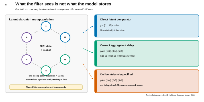
本專案把這個差異變成一個小型受控合成實驗。單一 deterministic 六區 SIR trajectory 提供隱藏 truth；四個比較 arms 使用同一條 truth、同一個 96-member prior ensemble、同一個動力系統、同一組 seeds、同一批 assimilation dates 及同一段 held-out horizon。它們唯一不同之處，是資料是否進入 filter，以及進入時所用的 observation operator：open loop 完全不更新；direct latent comparator 不切實際地看見六個感染狀態；目標 arm 使用預先申明的鄰區聚合、報告延遲、呈報比例與雜訊；misspecified arm 則用錯誤分組、沒有延遲及錯誤呈報比例，解讀同一條 aggregate stream。

若只看 point estimates，結果相當吸引。日數 0–44 之間，open loop 的 infected-state RMSE 是 $264.26$ ；正確 aggregate-and-delay operator 降至 $36.09$ ；錯誤 operator 則是 $126.34$ 。正確 arm 在沒有再接收觀察的 held-out 區間預測到真正峰值日，峰值強度誤差只有 $0.743\%$ ；錯誤 arm 遲五日，強度誤差 $4.726\%$ 。正確 arm 的 mean normalized innovation squared 是 $0.959$ ，落在固定的合理區間內。

但 uncertainty 結果沒有通過。名義上的 90% infected-state interval，在固定的 state-time comparison 中只覆蓋 $0.562963$ ，低於預先申明的最低門檻 $0.70$ 。五個核心 recovery criteria 中四個通過，coverage criterion 失敗，所以最後狀態必須是 PARTIAL，不能寫成 fully supported。RMSE 漂亮、平均 innovation 合理、peak forecast 準確，都不能抹去 latent uncertainty 的系統性 undercoverage。

本文所有數據均為 synthetic。「epidemic」、「reporting」與「forecast」只描述一個受控的六區數學 benchmark。沒有使用登革熱資料、病人紀錄、行政區個案、醫院報告、公共衞生介入或資源配置資料，也沒有臨床或政策建議。本實驗只用來說明 observation operator 如何改變 state recovery，並不驗證任何實際疫情系統。

比較結果顯示了甚麼

問題	結果	為何重要
研究背景	EnKF epidemic forecasting 與 observation-function effects 已有成熟工作	本文是一個聚焦的教學 benchmark，不是新的 filtering method。
Truth	deterministic 六區 SIR，每區 10,000 人	一條合成 latent trajectory，不是 fitted disease model。
Prior	共用 96-member ensemble 與固定 seeds	四個 arms 的初始 uncertainty 完全配對。
Assimilation	第 2 至 44 日，每兩日一次	單一 frozen update schedule。
Holdout	第 44 至 100 日	第 44 日後不再同化任何 observation。
Correct stream	三組相鄰區 incidence sums；0/1/2 日 weights $(0.15,0.35,0.50)$ ；reporting fraction $0.62$	Operator 由建構時已知，不是由數據估計。
Wrong stream	非相鄰分組、無延遲、reporting fraction $0.82$	刻意的 joint misspecification，不是另一個 fitted model。
Point recovery	五個 recovery checks 中四個通過	正確 operator 改善 state means 與 held-out peak forecast。
Uncertainty failure	90% state coverage $0.562963<0.70$	目標 arm 在固定 latent-state comparison 中 underdispersed。

這個比較防止數種偷換概念。Direct latent arm 不是實務上應選的方案，而是看見隱藏狀態後形成的 optimistic ceiling。正確 arm 的 innovation statistic 合理，不代表 latent intervals 已校準。研究動機與 dengue surveillance 有關，也不會把合成六區結果變成登革熱證據。

文獻如何改變研究問題

Ensemble data assimilation 在流行病模型中的應用早已建立。Evensen 在 1994 年奠定 sequential ensemble construction 的基礎（DOI）；Anderson 的 ensemble adjustment Kalman filter 則提供一個廣泛使用的 deterministic alternative 與 sampling diagnostics（DOI）。因此，本地 implementation 不能聲稱發明 ensemble filtering。

在 infectious-disease work 中，Shaman 與 Karspeck 已展示 ensemble-filter influenza forecasting（DOI）；Yamana、Kandula 與 Shaman 建立 dengue outbreak superensemble forecasts（DOI）；Pei 等人同化 spatial metapopulation influenza model（DOI）；Liu 等人亦把 EnKF 與 global spatiotemporal epidemic system 結合（DOI）。這些文獻排除了「EnKF 加空間疫情預測」本身的新穎性。

與本文最接近的重疊更直接。Mitchell 與 Arnold 專門研究 epidemic EnKF 的 observation-function selection，包括 incidence/prevalence mismatch 及 under-reporting（DOI）。這篇工作足以令「observation operators matter」不能被包裝成新發現。Cocucci 等人亦使用 ensemble data assimilation，讓 coarse epidemiological aggregates 約束較豐富的 hidden agent state（DOI）。

Reporting delay 同樣是既有的 measurement problem。Bastos 等人建立明確修正 delay 的 disease-surveillance nowcasting framework，並包含 dengue applications（DOI）；Yang 等人在 Bayesian epidemic assimilation 中使用 delay convolution（DOI）。Bretó 等人形式化 partially observed mechanistic systems 的 plug-and-play inference（DOI）；King 等人則展示 process 及 measurement errors 可產生 biased、overconfident 的 outbreak inference（DOI）。

所以文獻結論只能是 REFRAME。可辯護的貢獻不是新 filter、新 dengue model，亦不是首次發現 reporting process 重要；它是一個透明的 synthetic stress test：truth、prior、dynamics、seeds 與 update schedule 全部固定，只比較四條 observation pathways，並在看結果前申明 state、calibration 與 held-out peak gates。

更精確的研究問題是：

在一個固定六區合成系統中，已知的 aggregate-and-delay observation operator，相對 open loop 與刻意錯誤的 operator，可恢復多少 latent state 與 forecast performance；而其 uncertainty 是否通過預設 calibration gate？

最後一句不能刪掉，否則漂亮 RMSE 便可能遮住 overconfident ensemble。

模型儲存甚麼

每個 patch $i$ 包含 susceptible、infected、recovered 三個狀態。一般的 metapopulation SIR 可寫成

\frac{dS_i}{dt}=-\lambda_i(t)S_i, \qquad \frac{dI_i}{dt}=\lambda_i(t)S_i-\gamma I_i, \qquad \frac{dR_i}{dt}=\gamma I_i.

Force of infection $\lambda_i$ 透過固定 ring-mixing matrix 結合本區與相鄰區的 infected fractions。每區人口 10,000，本區 mixing weight 是 $0.76$ ，左右鄰區各是 $0.12$ ；patch-specific transmission coefficients 由 $0.22$ 至 $0.24$ ，recovery rate 是 $0.105$ 。這些無因次／日尺度參數只產生一條 pedagogical trajectory，不是任何病原體或城市的估計值。

Truth 的初始 infected counts 是 $(25,10,3,1,0.5,0.2)$ ；prior ensemble 則以 $(9,14,6,2,1,0.5)$ 為中心。Transmission-scale multiplier 的 prior mean 是 $0.78$ ，truth 是 $1$ ，所以 filter 面對真實而明顯的 state 與 parameter error，並非由近乎正確的 prior 開始。

模型另外保存三格 incidence queues，使 0/1/2-day report 可以直接寫成 augmented state 的 function。這個細節非常重要：delay 不是畫圖時把曲線平移，而是 latent dynamics 到 observation space 的 mapping 本身。

六區 latent SIR ring 及三條觀察路徑：不切實際的 direct latent counts、帶報告延遲的正確相鄰分組、以及無延遲的錯誤分組。 — 四個 arms 共用 truth、model、prior 與 seeds，只有 observation stream 或 operator 改變。Direct arm 是刻意不切實際的上限；wrong arm 用錯誤假設解讀同一 aggregate stream。

Filter 實際看見甚麼

Observation operator $h$ 把 latent state vector $x$ 映射至可量度空間：

y_k=h(x_k)+\varepsilon_k, \qquad \varepsilon_k\sim\mathcal N(0,R).

若 observation 是線性的，便有 $h(x)=Hx$ 。本實驗把 reporting queues 明確放進 state，因此 aggregate pathway 亦可由 augmented state 的 linear extraction 表示。核心不是矩陣是否線性，而是 $H$ 絕對不是 identity matrix。

Direct latent comparator 以 Gaussian standard deviation 18 觀察六個 $I_i$ 。它回答「若幾乎直接把 hidden state 交給 filter，algorithm 能做得多好」，適合作 diagnostic ceiling，卻不是可實施的 reporting design。

Correct aggregate-and-delay arm 觀察三組相鄰 pair sums： $(1+2)$ 、 $(3+4)$ 、 $(5+6)$ 。每組報告把 current 及前兩格 queue entries 按 $(0.15,0.35,0.50)$ 結合，再乘 reporting fraction $0.62$ ；Gaussian observation standard deviation 是 9。

Misspecified arm 收到完全相同的 noisy aggregate observations，卻用非相鄰 groups $(1+4)$ 、 $(2+5)$ 、 $(3+6)$ 解讀，假設 weights 是 $(1,0,0)$ ，即沒有 delay，並把 reporting fraction 改成 $0.82$ 。Grouping、delay 與 fraction 一次過共同改變，所以它只展示 joint misspecification 的損害，不能分辨三者各自的 causal contribution。

Open loop 只傳播同一 ensemble，不作 analysis update。它顯示 biased prior 在沒有資料時如何偏離 truth。

一個精簡的 EnKF update

令 $x_k^{f,(m)}$ 是更新時刻 $k$ 的第 $m$ 個 forecast ensemble member，forecast mean 為 $\bar x_k^f$ 。把 observation operator 套用到每個 member，得到 $y_k^{f,(m)}=h(x_k^{f,(m)})$ 。Ensemble anomalies 估計 forecast–observation 及 observation–observation covariance。Stochastic EnKF update 可以寫成

x_k^{a,(m)} =x_k^{f,(m)} +K_k\left(y_k+\varepsilon_k^{(m)}-y_k^{f,(m)}\right),

其中

K_k=P_{xy,k}^f\left(P_{yy,k}^f+R\right)^{-1}.

若 $h$ 錯了，innovation $y_k-y_k^f$ 便會在錯誤座標中被解讀。由 reporting delay 造成的差異可能被當成 current-state error；pair total 可能把 correction 推向錯誤 patches；reporting-fraction error 又可能被 transmission multiplier 或 infected counts 吸收。Kalman algebra 可以完全照公式執行，而 measurement semantics 仍然錯誤。

每次 analysis 後，implementation 把 epidemiological components 投影至非負值、重新正規化使每區 $S+I+R$ 等於人口，並把 transmission multiplier 限制在 $[0.45,1.55]$ 。這些 safeguards 保持 synthetic state 的 physical feasibility，但不是 posterior correctness 的證明。

四組配對比較

四個 arms 都在第 $2,4,\ldots,44$ 日同化，之後不再接收 observation，直接 forecast 至第 100 日。Prior ensemble 有 96 members；prior、direct observations、aggregate observations 及各 arm 的 propagation/update perturbations 均使用分開而固定的 seeds。沒有任何 arm 在看見 final truth 後再調參。

Assimilation-window metrics 包括：所有 patches 與 days 的 infected-state RMSE、mean spatial correlation、empirical 90% interval coverage、interval width、final transmission-scale bias 與 coverage，以及 mean normalized innovation squared。Held-out metrics 則包括 total-infected RMSE、total interval coverage、peak-day error 與 peak-intensity relative error。

Truth 的 total-infected peak 是第 62 日的 $12{,}025.316$ 。因 observation 在第 44 日停止，peak accuracy 確實沒有被其後 sequential updates 偷看；但它仍然屬於同一 synthetic model family，不能當作外部資料驗證。

四個 panels 比較 open loop、direct latent、正確 aggregate-delay 與錯誤 observation operator 在 assimilation window 內的 patch-one truth、ensemble mean 及 90 percent interval。 — 正確 aggregate-and-delay operator 大幅降低 point error，但 all-patch empirical 90% state coverage 只有 0.563。圖中同時展示 location 與 uncertainty，沒有隱藏失敗 gate。

Point recovery：顯著改善，但仍不及 direct arm

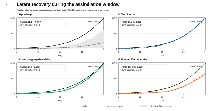
Open loop 的 assimilation-window infected-state RMSE 是 $264.255$ ，mean spatial correlation $0.8068$ ，coverage $0.3593$ 。帶偏 prior 在沒有 data updates 時無法跟上增長中的 latent field。

Direct latent observations 把 RMSE 降至 $11.677$ ，spatial correlation 升至 $0.9601$ ，coverage 是 $0.7481$ 。這建立一個 optimistic comparator：其 RMSE 是 correct aggregate arm 的 $0.3236$ 倍，低於固定的 $0.8$ ratio。這項比較在 information content 上刻意不公平，所以不能被寫成 deployable alternative。

Correct aggregate-and-delay arm 的 RMSE 是 $36.090$ ，spatial correlation $0.8523$ 。它的 RMSE 只是 open loop 的 $0.1366$ ，亦只是 wrong arm 的 $0.2857$ ，兩個 point-recovery gates 都大幅通過。Assimilation 結束時，transmission multiplier mean 是 $0.99321$ ，bias $-0.00679$ ；90% interval $[0.95534,1.02533]$ 包含 truth $1$ 。

Wrong operator 的 RMSE 是 $126.335$ ，spatial correlation $0.8525$ ，transmission-scale bias $-0.03108$ 。它仍可捕捉若干整體 spatial co-movement，所以 correlation 與 correct arm 很接近；然而 amplitude、uncertainty 與 forecast 全部較差。這提醒我們：去掉 level 與 scale 後的 correlation 可以看似有利，並不代表 absolute state recovery 良好。

Correct arm 仍然無法找回所有資訊。把六區壓縮成三個 pair totals，會失去每個 pair 內的分配；delay 混合近日 incidence；noise 與有限 ensemble size 進一步降低 identifiability。即使 observation process 在建構上完全已知，它的 state RMSE 仍約為 direct arm 的三倍。

Coverage 為何失敗

Nominal coverage 不是裝飾用的 uncertainty band。對每個受審核 patch-day state，protocol 檢查 truth 是否落在 ensemble 第 5 與第 95 百分位之間。有限且相關的樣本不必剛好得到 $0.9$ ；所以 protocol 已預先給出寬闊 admissible band $[0.70,0.99]$ 。低於 $0.70$ 視為 material undercoverage，高於 $0.99$ 則會提示 interval 過寬。

Correct arm 只覆蓋 $0.562963$ 的 state-time points。Mean interval width 雖有 $48.21$ ，latent error 增長後仍使大量 truth 落在 interval 外，因此 G4 明確失敗。

同一時間，mean normalized innovation squared 是 $0.9591$ ，落在 frozen interval $[0.25,2.5]$ 內。兩項 diagnostic 並不矛盾。NIS 在三維 observed aggregate space 中，以 predicted observation covariance 評估 innovations；state coverage 則在六個 patches 的 latent infected values 上，跨時間檢查十八維 hidden components。Aggregate residuals 可以看似合理，而 observed pair 內部如何分配的 conditional uncertainty 仍被低估。

這正是 benchmark 最重要的發現：observation-space calibration 不能自動證明 latent-state calibration。Filter 可以解釋它看見的東西，同時對無法分開觀察的量過度肯定。

Held-out peak forecasts

第 44 日之後，所有 arms 都沒有新 observations。Open loop 把 peak 預測遲 21 日，intensity error $57.857\%$ ，total-infected holdout RMSE $5364.98$ 。Direct latent arm 預測正確 peak day，intensity error $0.221\%$ ，holdout RMSE $15.65$ 。

Correct aggregate-and-delay arm 同樣預測真正的第 62 日峰值；peak-intensity relative error 是 $0.743\%$ ，holdout RMSE $59.59$ 。Misspecified arm 遲五日，intensity error $4.726\%$ ，holdout RMSE $1493.71$ 。故此 correct operator 通過 frozen G6：其 absolute timing 與 intensity errors 均不差於 wrong operator。

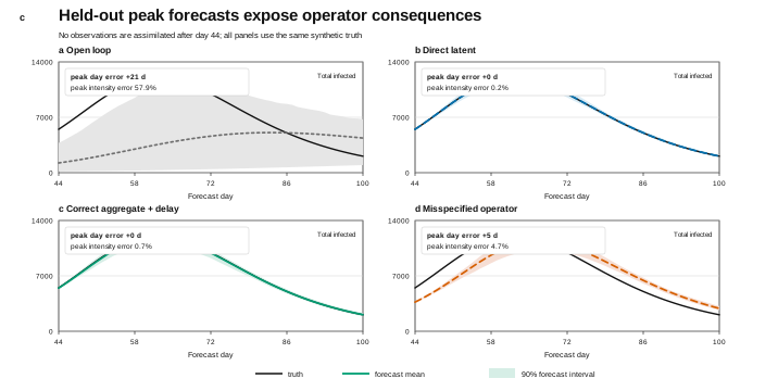
由第 44 至 100 日的四個 held-out total-infected forecast panels，比較 truth 與 open-loop、direct-latent、正確 aggregate-delay、misspecified-operator ensemble，並列出 peak errors。 — 第 44 日後不再同化 observation。正確 operator 保留真正第 62 日峰值，強度誤差 0.743%；錯誤 operator 遲五日，強度誤差 4.726%。

Correct 與 direct arms 的 held-out total 90% coverage 都是 $1.0$ ，但這不能抵銷 assimilation state undercoverage。Total infected 是跨 patches 的加總，holdout interval 又屬另一個時間窗口與另一個 functional；patch-level errors 可以在加總中互相抵銷，total interval 亦可能夠寬而容納 truth，即使不少 individual latent states 被漏掉。

比較結果如何判定

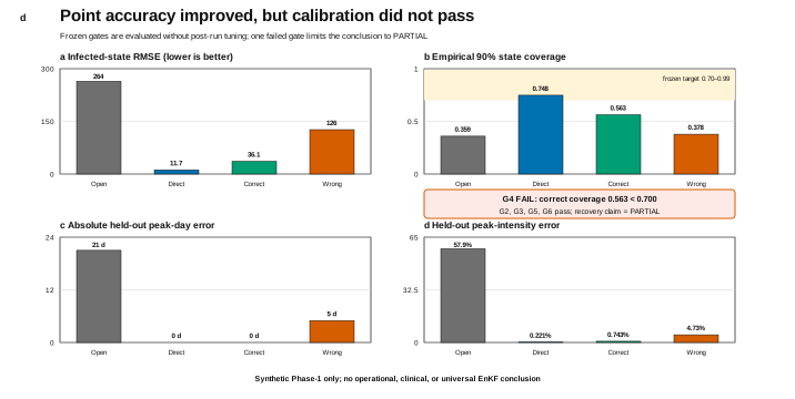
比較使用六項預先指定的準則。G1 提供背景對照：direct latent RMSE 必須不高於 correct-operator RMSE 的 $0.8$ 倍，才可視作 optimistic comparator；觀察值 $0.3236$ ，所以通過。

五個核心 recovery gates 是：

G2： correct RMSE / open RMSE $\le 0.85$ ；觀察值 $0.1366$ ，通過。
G3： correct RMSE / wrong RMSE $\le 0.8$ ；觀察值 $0.2857$ ，通過。
G4： correct state coverage 必須在 $[0.70,0.99]$ ；觀察值 $0.562963$ ，失敗。
G5： correct mean NIS 必須在 $[0.25,2.5]$ ；觀察值 $0.9591$ ，通過。
G6： correct peak-day 與 intensity errors 不得差於 wrong；觀察值 $0$ 日及 $0.743\%$ ，相對 $5$ 日及 $4.726\%$ ，通過。

固定規則要求五項全部通過，才可作出完整 recovery statement。本次四項通過，所以 point 與 peak improvement 仍然成立，但更強的 calibrated-recovery statement 不成立。

四個 panels 比較 open、direct、correct、wrong observation arms 的 infected-state RMSE、empirical 90 percent state coverage、held-out peak-day error 與 peak-intensity error，並突出失敗的 coverage gate。 — Point accuracy 與 held-out peak performance 改善，但預設 state-coverage target 沒有通過。這項 uncertainty failure 令完整 recovery claim 不成立。

這條規則阻止常見的修辭捷徑：只刊登成功的 RMSE 與 forecast panels。Uncertainty failure 是同等重要的 evidence，不能變成補充資料中的小字。

為何幾項 metrics 會得出不同印象

四項主要 diagnostics 回答不同問題，不能壓成一個單一分數。RMSE 問 ensemble mean 在 infected-count 單位上是否接近 latent truth；spatial correlation 問六區 pattern 在移除大部分 level 與 scale information 後是否同步起伏；empirical coverage 問 ensemble 所申報的 uncertainty 是否以承諾頻率容納 truth；NIS 問三維 observed aggregate space 中的 residual，相對 predicted observation covariance 是否合理；held-out peak functional 又問未來 total 的 derived event，而不是每個 latent component。

這張 crosswalk 解釋幾個看似奇怪的結果。Wrong arm 的 correlation $0.8525$ 可略高於 correct arm 的 $0.8523$ ，但 RMSE 卻超過三倍。Correct arm 的 NIS 可是 $0.9591$ ，latent coverage 仍只有 $0.563$ 。Correct 與 direct arms 的 held-out total coverage 可全部命中，而 correct arm 在 assimilation 期間仍漏掉很多 patch-level states。這些差異不是讓研究者挑最漂亮的 metric，而是說明每項 metric 只是 partially observed system 的不同投影。

所以 verdict 亦不是看完表格後才設計的 weighted average。Protocol 給 state-coverage gate 對 fully supported recovery claim 的 veto。未來研究若只重視 peak timing，可以預先申明另一個 estimand 與 decision rule；但不能在本次 gate 失敗後，把原來的 uncertainty target 改名為不重要。

正確 operator 為何仍會 undercover

以下幾種機制都可產生目前 pattern，但本實驗沒有逐一識別因果。

第一，aggregation 消滅對比資訊。同一 adjacent-pair total 可由兩區之間很多不同分配產生。Cross-patch dynamics 有助重建，但不等於直接量度。

第二，delay 混合時間。某個 assimilation date 的 observation 同時包含 current 與前兩個 queue entries。即使 weights 正確，反演仍帶有 noise，連續 updates 之間亦相關。

第三，finite ensemble 只近似 covariance。96 members 要估計高維 augmented covariance，弱觀察 directions 的 uncertainty 可能被低估。本實驗沒有測試 localization、inflation、更大 ensemble 或 smoother。

第四，projection 改變 distributions。Nonnegativity、population conservation 與 parameter bounds 在物理上合理，但 nonlinear projection 可以改變 spread 與 Gaussian assumptions。

第五，truth 與 filter 共用 model family。目標 arm 沒有 structural process mismatch，屬於相對有利的 closed world。若連這個環境也出現 undercoverage，更合理的反應是提高警覺，而不是把精確 intervals 外推到現場。

這些是 plausible explanations，不是實驗已分辨的 causes。後續 phase 必須預先申明 ensemble-size、inflation、localization、smoothing 與 aggregation ablations，才可討論哪個修改真正改善 calibration。

Wrong arm 能說明甚麼，又不能說明甚麼

Wrong arm 同時改變 spatial grouping、delay 與 reporting fraction。較差的 RMSE、forecast 與 coverage 證明這個 composite mismatch 在 frozen design 中有實質後果；它不能告訴我們三個因素誰最重要，也不能證明所有錯誤 operators 永遠較差。某些 wrong models 在特定 truth 下可能碰巧互相補償。

其 mean NIS 是 $2.4737$ ，仍剛好位於上限 $2.5$ 內，state coverage 卻只有 $0.3778$ ；holdout total coverage 更跌至 $0.1754$ 。再一次，aggregate observation-space average 不保證 latent calibration。Wrong arm 的 spatial correlation 又可比 correct arm 高一點，但 level error 與 forecasts 明顯較差。這正是 multi-metric gates 必要的原因：每項 statistic 都有 blind spot。

本 benchmark 沒有建立的結論

下列說法全部超出 evidence：

某個真實 dengue surveillance system 正在使用或應該使用本文 operator；
六個 synthetic patches 對應某些行政區、醫院或社群；
Delay weights 與 reporting fraction 符合任何 field records；
EnKF 優於 particle filters、smoothers、variational methods 或 Bayesian alternatives；
修正 observation operator 便必然得到 calibrated latent uncertainty；
Transmission multiplier 具有現實 epidemiological interpretation；
Held-out peak 是 operational forecast；
結果可用來作 intervention、resource allocation 或 health decision；
Joint misspecification experiment 已識別每個 component 的個別效應；
單一 deterministic synthetic truth 足以證明 general robustness。

本文沒有使用任何真實人物或 case record，亦沒有 clinical、public-health 或 policy readiness claim。

從線性代數看「看不見」的方向

聚合觀察為何不能自動還原逐區狀態，可以用一個很簡單的例子理解。假設第一個觀察只提供第一區與第二區的總和，忽略延遲後可寫成 $y=I_1+I_2$ 。狀態 $(I_1,I_2)=(40,60)$ 與 $(55,45)$ 都給出同一個觀察 $y=100$ 。只要把第一區增加的量，等量從第二區減去，觀察便完全不變。向量 $(1,-1)$ 因此位於該聚合算子的零空間：沿這個方向移動，儀器看不到任何差別。

六區變成三個相鄰總和時，每個配對都存在相似的區內對比方向。動力模型、跨區傳播與不同時刻的資料，可以間接限制這些方向，但不能把間接推斷變成直接量度。若 ensemble covariance 對這些弱觀察方向估得太窄，pair totals 仍可配合得很好，而 individual patches 的 truth 已經跌出區間。這正好對應本次「觀察空間的平均殘差合理、隱藏狀態覆蓋不足」的組合。

延遲令問題再多一層。現在的報告不只對空間做加總，亦把三個相鄰日子的 incidence 按固定權重混合。某個較高報告可以來自今天較高、昨天較高，或前日較高；動力方程會限制可能組合，但噪聲與有限更新頻率仍留下時間方向的不確定性。故此，正確算子只表示 filter 沒有故意使用錯誤 measurement equation，不等於 inverse problem 已變成唯一且容易。

這也解釋 direct arm 的角色。它近乎逐區直接觀察 $I_1,\ldots,I_6$ ，大幅削弱上述零空間，所以可作為「若資訊非常充足，現有 algorithm 是否能跟上 truth」的實作診斷。它與正確 aggregate arm 的差距主要反映資訊條件不同，不能被改寫成「實務上應該收集不存在的 latent counts」。

逐步追蹤一次錯誤更新

想像真實報告在某一日上升，原因是前兩日的 incidence 經延遲權重累積，並在相鄰第一、二區合併後出現。正確 arm 先用同樣的三日佇列與相鄰分組，為每個 ensemble member 產生 predicted observation；其 innovation 代表「在相同報告機制下，預測總量與收到總量相差多少」。Kalman gain 再依樣本 covariance，把 aggregate discrepancy 分配回逐區狀態、近期 incidence queues 與 transmission multiplier。

錯誤 arm 看見相同數值，卻假設沒有延遲。它會把本來由過去 incidence 造成的上升，較多當成今日 latent state 的不足。它又把第一區與第四區配對，所以 correction 可能推向不應共同調整的空間位置；呈報比例由真實建構的 $0.62$ 誤設為 $0.82$ ，則令同一報告被解讀成較小的 underlying incidence。三種錯誤可互相影響，filter 甚至可能以改動 transmission scale 來補償 observation equation 的偏差。

一次更新後，兩個 arms 都會保持非負與人口守恆，看上去數值穩定；錯誤 arm 的曲線亦可能跟隨整體上升趨勢，令 correlation 不差。可是物理可行、趨勢相似與 measurement semantics 正確是三個不同判準。累積多次更新後，小偏差會進入 day-44 initial condition，再傳播至沒有新資料的 holdout，因此 wrong arm 最後出現五日 peak delay 與顯著較大的 forecast error。

這個逐步故事只是對既定機制的解讀，不是另一次數值實驗。本研究沒有把三種錯誤單獨開關，所以不能用目前數值量化「哪一種錯誤貢獻幾多百分比」。它的用途，是提醒讀者不要把一句「operator wrong」理解成單一 scalar parameter 偏差。真正的 attribution 至少要分開改動 grouping、delay 與 reporting fraction，再加入事前指定的交互組合；否則任何單因歸因都超出這次比較。

四幅圖各自回答甚麼

第一幅圖是 protocol diagram，不是結果圖。讀者應先確認左方 hidden state 與右方三條 observation pathways 的資訊量不同；direct comparator 的虛線箭頭不能與可實施的 aggregate stream 混為一談。圖底亦明確寫出 synthetic truth、共用 prior 與 frozen seeds，避免把 arm 差異歸因於不同初始抽樣。

第二幅圖只展示第一區曲線，但 callout 的 RMSE、相關與 coverage 是所有六區共同計算。因此不能由單一 panel 的視覺貼合，推斷全場 coverage 已通過。Open loop 的灰色帶很寬仍漏掉快速增長 truth；correct arm 的綠線接近 truth，卻仍有很多區時點不在 interval 中。這正是數值摘要必須與曲線並讀的原因。

第三幅圖轉到 day 44 之後的 total infected。每個 panel 共用同一 truth，而且不再 assimilate observations；所以 peak-day comparison 是真正的 protocol holdout。可是 total 是六區加總，與第二幅圖的 patch-level states 不是同一 estimand。若只看到 correct arm 的 peak 幾乎吻合便宣布 uncertainty 成功，就會跨越圖與圖之間的定義界線。

第四幅圖把四個判斷放在同一面板：左上比較 RMSE，右上比較 state coverage，左下是 peak-day error，右下是 peak-intensity error。黃色範圍標出 coverage 的固定目標，紅框則把 G4 failure 放在 point 與 peak improvements 旁邊。不能只比較柱高而忽略每一格回答的問題不同。

為何單一合成 truth 只能回答窄問題

固定一條 truth 有明顯優點：每個 arm 遇到完全相同的 epidemic trajectory，差異不會被不同真值或 seeds 混淆；所有 metrics 亦可逐位重算。這種設計適合核對數值行為及比較 observation mechanism，尤其可確認各 operators 是否按同一套規則讀取同一 stream。

限制同樣明顯。某個 operator 在這條 trajectory 上改善，不代表在不同初始感染位置、傳播速度、mixing strength、delay kernel、reporting fraction 或 noise level 下仍保持相同排序。Peak 在第 62 日、assimilation 在第 44 日停止，也是單一幾何關係；若 peak 更早、更平或有多峰，forecast metrics 可能改變。固定 ring topology 亦沒有涵蓋稠密、稀疏、方向性或時間變動 network。

因此，重複計算一致的意義只到「相同輸入會產生相同輸出」。它不等於 Monte Carlo robustness，不等於跨 model class validity，更不等於 field generalisation。下一階段若要談穩健性，應先建立多個預先生成而不因結果篩選的 truths，為每個情境保留個別 failure，再報告分布而不是只報平均。若要談現實資料，則要另外處理真值不可見、報告修訂、缺失、空間邊界改變與參數不可辨識；不能把 synthetic truth 的可得性偷偷帶入現場敘事。

門檻的作用不是把連續數值假裝成自然定律。Coverage 下限 $0.70$ 、NIS 範圍與 RMSE ratios 都是本次比較的決策規則，讓「甚麼結果足以支持哪一句話」在看到結果前已清楚。另一個研究團隊可以選擇更嚴格門檻，但應在新實驗前解釋用途、誤判代價及容許的 uncertainty。本文只按自己的固定規則解讀結果，不把這些數字當成所有資料同化工作的普遍標準。

通過四項檢查也不代表獲得「五分之四的真理」。Coverage 對 calibrated-recovery statement 是必要條件，不能由較好 RMSE 抵銷。這使後續研究知道應把資源放在 uncertainty representation，而不是繼續美化已經不錯的 point estimate。

數值核對能建立甚麼

以相同輸入重複計算，得到相同 state histories、metrics 與 coverage failure。Population conservation、nonnegativity、observation dimensions 及 aggregate-and-delay calculation 亦符合各自的數學定義。這些數值結果支持目前比較，卻不會增加其 empirical scope。

一個重複得到的 synthetic result 仍然是 synthetic。兩次一致，只表示 undercoverage 不是這次 calculation 的單次偶然；它不能證明不同 truth、parameters、networks 或 reporting mechanisms 下仍會保持同一排序。那些問題需要新的 experiment family。

改善了甚麼，又有甚麼仍未解決

這個結論不是好壞印象的平均。正確 operator 相對 open loop 與 wrong mapping，確實改善 state point estimates，亦得到合理 mean innovations 與準確 held-out peak；這些 narrow claims 在 benchmark 內有支持。可是同一 ensemble 沒有達到最低 state coverage，所以「以 calibrated uncertainty 恢復 latent field」這個更廣闊 statement 不獲支持。

寫成「正確 operator works」會過度概括；寫成「正確 operator fails」又會丟棄真正的 point 與 forecast improvement。最精確的結論是：

在這個固定 synthetic experiment 中，明確建模已知的 aggregation 與 delay，可恢復不少因 partial observation 而流失的 point 與 peak performance；但 latent infected states 的 ensemble 仍然 underdispersed。

這句話同時保存兩方面的結果，亦沒有 operational extrapolation。

下一步應測試甚麼

新 protocol 應研究 coverage failure，而不是事後把它調走。候選 frozen axes 包括 ensemble size、inflation、localization、iterative updates、fixed-lag smoothing、delay-kernel uncertainty、reporting-fraction estimation、pairwise 與 larger aggregation，以及 controlled process mismatch。每個 change 應在多條 held-out synthetic truths 上評估，而不是只用一個 seed family。

最清楚的設計可分成兩層。第一層固定 observation operator，只改 uncertainty representation：例如 48、96、192 members，配合數個事前指定的 inflation levels，並比較有無 localization 與 fixed-lag smoothing。每個設定都在同一批預先生成的 truths 上運行，逐條保存 patch-level coverage、observation-space NIS、interval width 與 peak error。若 coverage 改善但 intervals 變得過闊，結果便應如實顯示 trade-off，而不是只報較高命中率。

第二層固定 filter setting，把 grouping、delay kernel 與 reporting fraction 分開改變。可以先逐一改一項，再加入事前指定的二因子 combinations，判斷錯誤是近似相加，還是會由 transmission multiplier 的補償而互相抵銷。Correct stream 與所有 wrong interpretations 必須繼續使用同一 noisy observations，否則 data realization 的差異會混入 operator effect。

多條 truth 亦不能只換 random seed。初始感染位置、transmission scale、ring mixing strength、peak timing、delay weights 與 noise level 應按預設格點或分層設計改變。報告要同時列出每條 truth 的 failure，而非只給平均 RMSE；否則少數嚴重 undercoverage 可被大量容易 cases 沖淡。這樣才可判斷目前 $0.562963$ 是某條 trajectory 的特殊幾何，還是多種 partial-observation settings 中反覆出現的模式。

如何分辨 calibration 改善與單純加闊區間

最直接的修補是增加 ensemble spread，例如 multiplicative inflation；但 interval 變闊自然會提高 coverage，所以單看 coverage 上升不足以判定方法更好。下一個實驗應同時報告 interval width、RMSE、NIS 與一個事前指定的 proper scoring rule。若 coverage 由 $0.563$ 升到目標範圍，但 width 擴大至失去決策價值，這是 coverage 與 sharpness 的交換，不應寫成無條件 improvement。

Calibration 亦要按資訊方向拆開。每個 adjacent pair 的 total direction 被直接觀察，pair 內的 contrast direction 則主要靠 dynamics 與 covariance 推斷。可以把 error 和 interval coverage 投影到這兩類 directions，再看 inflation 是修復弱觀察 contrast，還是把所有方向一律放大。如果 NIS 仍接近一，而 contrast-space coverage 特別低，就比單一 all-state percentage 更接近本次 failure mechanism。

Localization 的測試也要符合六區 ring geometry。過強 localization 可能切斷真正跨區 transmission correlation；過弱則讓 finite-ensemble noise 把一個 aggregate report 傳到太遠 patches。合理設計應預先指定數個半徑，對每條 truth 比較 correction 在 observed pair、nearest neighbours 與遠端 patches 的分布，並檢查 population conservation 後 spread 是否被 projection 再次壓窄。

Fixed-lag smoother 回看近日 queue states，理論上更配合延遲報告，卻使用未來於當時不可得的 observations 來改善過去估計。故此 smoother result 必須與 filter result 分開命名。它可以回答 retrospective state reconstruction 是否改善，不能直接冒充 real-time forecast performance。Day-44 之後的 held-out peak 仍要由當時可用資訊出發，才保持原來 forecast question。

最後，calibration 不應只在全時段平均。感染初期 counts 低、增長段 steep、峰值附近 dynamics 轉向，三段的 observability 與 Gaussian approximation 都不同。分段 coverage curve 能指出 underdispersion 在何時形成，也能判斷某種修補只是推遲 failure，還是真正維持 uncertainty。這些 diagnostics 都應在新 truths 打開前固定，避免看到某段最漂亮才決定報哪一段。

目前 operator 由建構時完全已知，實際 surveillance 卻往往要估計 reporting fraction 與 delay weights。下一步若把這些量加入 ensemble state，interval 必須同時反映 parameter uncertainty 與 latent-state uncertainty；若先以全部資料估好 weights，再把它們當成固定真值，會低估兩階段 estimation 帶來的 spread。更嚴格的設計可用 training period 估計 reporting process，在 untouched period 同時檢查 observed reports、latent synthetic truth 與 peak forecast，並把 operator-parameter coverage 與 infected-state coverage 分開。這樣才可判斷較闊 uncertainty 是來自合理傳播 reporting ambiguity，還是 filter 本身失去辨識能力。

每次修補亦要保留 direct、correct、wrong 與 open-loop 四組比較。若只重跑 correct arm，coverage 上升可能來自較容易的新 truth，而非 uncertainty method；配對設計才能把這兩種解釋分開。

Attribution design 應把 grouping、delay 與 reporting fraction 分開及交互改變，辨認每種 misspecification 主要傷害哪一項 metric，並測試 interactions 是否近似 additive。Sensitivity panel 亦應分開 observation-space NIS、patch-level state coverage 與 total-field coverage。

只有在 synthetic calibration 理解清楚後，real-data work 才有意義。屆時需要 data provenance、reporting definitions、revision 與 delay process、privacy governance、適合該 disease 與 geography 的 model、parameter identifiability analysis、真正 out-of-sample periods 及 domain-expert review。那會是一個新 project，不是本 benchmark 的小附註。

結論

Data assimilation 並非直接吸收 reality，而是吸收 measurement model 的輸出。當 filter internal state 與 reporting system output 不同，observation operator 是 scientific model 的一部分，不是外圍 plumbing。

本次 frozen result 沒有製造成功故事。Known aggregate-and-delay operator 把 assimilation RMSE 由 open loop 的 $264.26$ 降至 $36.09$ ，優於 wrong operator 的 $126.34$ ，亦保存準確 held-out peak；但 nominal 90% latent-state interval 只覆蓋 $56.30\%$ ，所以完整 recovery claim 失敗。Direct latent arm 仍然只是 unrealistic upper benchmark；wrong arm 亦只展示 joint misspecification，不是 universal law。

方法上的實際教訓很簡單：送入同化器的應是 instrument 或 reporting process 真正可觀察的量；uncertainty 要在 observation space 與 latent space 分別評估；若 calibration gate 失敗，便讓它留在圖中與結論中。