網格能保留事件嗎？

這個實驗最值得寫下來的地方，是結果與直覺相反：給網格更多關於研究目標的資訊，並沒有令它在今次計算中更準確。在同樣使用 36 個 elements 的 production budget 下，uniform finite-element mesh 找到 modal transition 的時間，比 conventional residual mesh 及專為事件時間設計的 dual-weighted-residual（DWR）mesh 都要接近 reference。

獨立 cosine-spectral reference 把 transition 定在 $t^*_{ref}=46.7916$ 。Uniform mesh 得到 $49.3918$ ，absolute error 是 $2.6001$ ；DWR 得到 $50.0668$ ，遲了 $3.2752$ ；residual adaptation 得到 $51.1947$ ，遲了 $4.4030$ 。三者都超過預先定下的 1.5 time-unit error ceiling，因此 Phase 1 的決定是 REFRAME，而不是宣稱 uniform refinement 一般地優於 adaptive methods。

一次 coarse、one-shot comparison 不足以推翻 DWR。它揭示的反而是一個具體失敗機制：兩個 adaptive meshes 都由 24-element pilot 選出，但 pilot 本身的事件時間已經遲了約 7.19。它的 first-order DWR correction 更達到 $-80.336$ ，遠大於真正誤差。在這種線性化品質下，indicator 即使找到數學上相關的位置，也未必能把事件時間拉回正確位置。

這個實驗發現了甚麼

問題	結果	為何重要
Reference event 是否穩定？	$t^*_{ref}=46.7916$	比較有一個明確目標。
同時加密 space 與 time 後移動多少？	$0.000641$	Reference uncertainty 遠小於所有 FEM error。
Crossing 是否 transversal？	$\dot G(t^*)=0.0584$	Root 並非幾乎相切。
36 elements 下哪個最好？	Uniform，error $2.6001$	選擇性配置今輪沒有勝出。
DWR 表現如何？	Error $3.2752$ ，effectivity $2.686$	排第二，並高估誤差幅度。
Residual adaptation 表現如何？	Error $4.4030$	降低 field residual 不等於保護事件。
有沒有 FEM run 通過 error ceiling？	沒有	下一步應做 refinement ladder，而非包裝成成功。

這是一個刻意控制規模的 smoke experiment。它證明 reference、event derivative、三個相同大小的 production meshes，以及 error estimator 能在同一設計中運作；它尚未證明 asymptotic rate、cost advantage 或普遍的 method ranking。

Registered 與 refined reference 的局部線性化在幾乎相同時間通過零點。 — 同時加密 space-time 後的 crossing shift 很小；圖中兩條線是 local linearisation，並非完整 trajectory。

為何問題是事件，而不只是場的誤差

Reaction–diffusion simulation 直接輸出的是一個 field：兩種濃度如何隨空間及時間變化。但真正想回答的科學問題，往往是這個 field 何時改變性質，例如花紋何時多出一條 stripe、某個 spatial mode 何時取代另一個，或者 activation front 何時首次越過 threshold。這些都是 event questions。

Field accuracy 與 event accuracy 有關，卻不能互相取代。整體 norm error 看來不大，仍可能令 threshold crossing 明顯移位；相反，某些與 endpoint 無關的局部差異可以很顯眼，但關鍵 modes 的 crossing time 仍然正確。若問題是「何時發生」，只在 field residual 最大的位置加密，可能把 resolution 花在錯誤地方。

本研究使用 modal transition，而不用 peak count。令 $a_k(u)$ 表示 activator perturbation 的第 $k$ 個 cosine coefficient，事件 functional 是

G(u)=a_7(u)^2-a_6(u)^2.

Event time 定義為 $t=10$ 之後第一個由負變正的 transversal root：

t^*=\inf\{t\ge 10:G(u(t))=0,\ \dot G(t)>0\}.

Crossing 之前，mode 6 的 squared amplitude 較大；之後則由 mode 7 佔優。平方可以消除 modal sign 的任意性，而 transversal crossing 令局部 event time 可以微分。這個 endpoint 精確量度 spectral dominance 的轉移，不應被重新描述成已驗證的 topology split 或 biological landmark。

Peak count 看來直觀，但它對小 perturbation 不連續，也依賴 prominence、smoothing 與 shoulder 判定。一個很淺的局部峰已可令 count 改變。Modal equality 雖然仍是模型化選擇，卻提供一個清楚 scalar root，適合做 refinement 與 adjoint verification。

Growing-domain 模型

Benchmark 是一維 Schnakenberg reaction–diffusion system，定義在預先指定的 growing interval。把 physical coordinate 拉回固定 reference coordinate $\xi\in[0,1]$ 後，兩個濃度滿足

u_t=a-u+u^2v+\frac{D_u}{L(t)^2}u_{\xi\xi}-\frac{\dot L(t)}{L(t)}u,

v_t=b-u^2v+\frac{D_v}{L(t)^2}v_{\xi\xi}-\frac{\dot L(t)}{L(t)}v,

兩端使用 no-flux boundary conditions。參數為 $a=0.1$ 、 $b=0.9$ 、 $D_u=8\times10^{-4}$ 、 $D_v=2\times10^{-2}$ 。Domain length 包含慢速 exponential growth 與一個以 $t=45$ 為中心的 smooth pulse。當 $L(t)$ 增加，reference coordinate 中的 effective diffusion 會減弱，而 $\dot L/L$ dilution term 會隨擴張移除濃度。

這個設計同時包含兩種機制：reaction 與 diffusion 決定哪些 spatial modes 可以增長；domain growth 則改變 physical wavelength 與 effective diffusion scale。Growth pulse 令 mode 6 至 mode 7 的轉移在 60 time units 內出現。Initial perturbation 包含多個 cosine components，並使用固定 seed。這些都是 synthetic benchmark choices，並非由 biological data 擬合所得。

固定 reference coordinate 亦令比較更乾淨。位於 $\xi=0.4$ 的 node 會隨 $L(t)$ 在 physical domain 移動，但 reference label 不變，因此可以把 element placement 與 domain expansion 分開理解。

既有研究如何收窄問題

Growing-domain pattern formation 並非新題目。Crampin、Gaffney 與 Maini 已推導 growing domains 上的 reaction–diffusion equations，並研究 Schnakenberg system 的 frequency doubling。其後工作發展 moving-grid、evolving-domain FEM 與 finite-difference schemes，分析 convergence，亦指出 grid velocity 可以影響最後選出的 pattern。因此「growth 能改變 Turing pattern」和「FEM 能模擬它」都不是本研究的新貢獻。

Adaptivity 同樣有清楚前例。Semilinear reaction–diffusion residual estimators、growing-domain adaptive FEM，以及 goal-oriented methods 都已有文獻。Goal-oriented 方法的特別之處，是用與 quantity of interest 對應的 adjoint 去加權 residual。First-time-to-threshold functional 亦有專門的 error representation，因為移動一個 root 並不等同降低 state norm。

所以今次有意義的問題很窄：選定一個 smooth event，先建立 independent reference，再讓 uniform、residual 與 DWR 在相同 production DOFs 下比較，而且無論 goal-oriented method 是否勝出都保留結果。這是 controlled benchmark，不是任何單一 ingredient 的 novelty claim。

同一 transition 的兩個數值視角

Reference solver 刻意與比較中的 FEM solver 不同。它在 512 個 cell centres 上用 cosine modes，time step 是 $0.0025$ ，並以 Strang splitting 前進。Diffusion 在 cosine space 中是 diagonal，reaction 與 dilution 則用 second-order update。Reference refinement 同時把 cells 加倍與 time step 減半。

Production solver 使用 nodal continuous P1 finite elements，在每個候選 mesh 上獨立 assemble consistent mass 與 stiffness matrices。Reaction 與 dilution 採用相同 temporal order，diffusion 以 Crank–Nicolson 處理，time step 是 $0.02$ 。Event value 由 finite-element field 的 quadrature-based cosine projection 算出。

兩套 solver 共享 mathematical model、initial state 與 event definition，但不共享 spatial representation 或 diffusion update。它們的吻合可以降低某一個 assembly path 出錯的可能，卻不能排除兩者共同假設有誤，更不能代替 experimental validation。

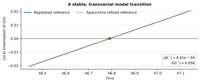
Reference crossing 是 $46.7916133$ ，refined value 是 $46.7909721$ 。兩者相差 $6.41\times10^{-4}$ ，比最佳 production error 小超過四千倍。Crossing slope 為 $0.058425$ ，遠高於預定 transversality floor $0.002$ 。換言之，今次 ranking 並非由未解像或近乎相切的 reference root 決定。

同一 budget 下的三個 meshes

每個 production mesh 都有 36 elements，亦即每個 scalar state 有 37 DOFs。系統包含兩個 variables，並走 3,000 個 steps，所以每次 production solve 都有 222,000 primal DOF-steps。這是 matched primal-work proxy，不是 matched wall-clock cost；adaptive strategies 另外需要 pilot、indicator、enriched adjoint 與 mesh selection overhead。

Uniform mesh 平均切分整個 interval，不使用 pilot-derived preference。Residual mesh 由 24-element pilot 開始，累積兩個 fields 的 flux-jump indicators，再把最高分 elements 切分至 36 個。DWR mesh 則解一個 enriched backward adjoint，其 terminal condition 來自 event-time sensitivity；它把 event 前的 space-time residual 乘以 adjoint，再按最大的 element contributions 加密。

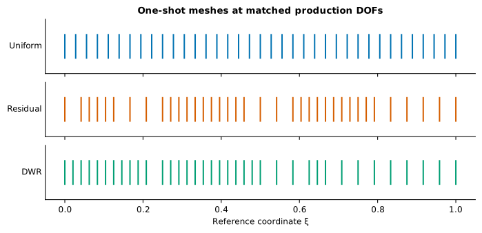
Uniform、residual-adapted 與 DWR-adapted 三個 one-shot meshes 的 node locations，每個均有 36 elements。 — 相同 element count 不代表相同 placement；residual 與 DWR 把同一 budget 集中在不同位置。

這些是 one-shot designs，並非重複 solve-estimate-mark-refine 直至 estimator convergence。這個限制是理解結果的核心。Goal-oriented method 依賴合理的 primal trajectory 與 adjoint linearisation；一個太粗的 pilot 未必足以預測下一個 mesh 真正需要甚麼。

Matched-work 比較結果

Uniform mesh 在兩個 reported errors 都最好。它的 event time 是 $49.3918$ ，遲 $2.6001$ ；relative final-field error 為 $0.1131$ 。DWR 的 event time 是 $50.0668$ ，遲 $3.2752$ ，field error 為 $0.1596$ 。Residual adaptation 得到 $51.1947$ ，遲 $4.4030$ ，field error 為 $0.1405$ 。

Uniform、residual 與 DWR 的 transition-time error，以及 event accuracy 與 final-field accuracy 的關係。 — 左圖是主要 endpoint；右圖說明 field-norm ranking 不能代替 event-time ranking。

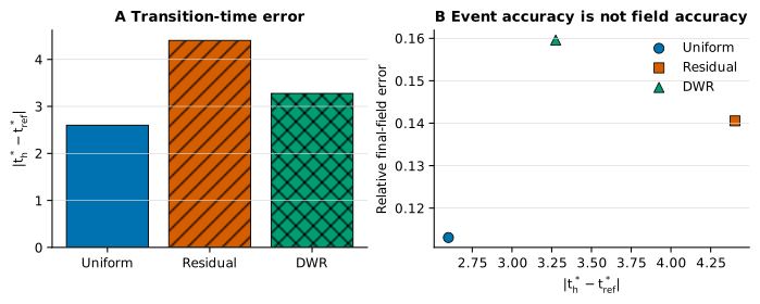
這些數字帶出兩點。第一，固定 coarse budget 下，adaptivity 不會自動有優勢。對一個 global cosine functional 而言，uniform coverage 可能較能保留整體 phase balance。第二，不同 endpoint 會產生不同 adaptive ranking。DWR 的 field error 比 residual 大，但 event-time error 較小，這與它的 goal-oriented 目的相符，只是仍未能勝過 uniform。

三個 production runs 都找到事件，沒有 missed event。失敗是 quantitative 而非 categorical：事件存在，但所有 FEM times 與 reference 相差都超過 1.5。這個 ceiling 在看到排名前已固定，所以正確處理是 REFRAME，而不是把「最不差」包裝成成功。

Adjoint 驗證了甚麼

對 transversal root $G(u(t^*))=0$ ，perturbation $\delta u$ 對 event time 的 first-order 影響是

\delta t^*=-\frac{G_u(u(t^*))\,\delta u(t^*)}{\dot G(t^*)}.

這條式一方面提供 backward adjoint 的 terminal quantity，另一方面亦給出直接 verification target。對預先指定的 modal perturbation，analytic event-time derivative 是 $2.77896594$ ；centred finite difference 是 $2.77896596$ ；relative difference 只有 $8.24\times10^{-9}$ 。

三個 meshes 的 estimator effectivity，以及 adjoint 與 finite-difference event-time sensitivity 的核對。 — Derivative check 極為接近，但三個 estimators 都高估實際 event-time error magnitude。

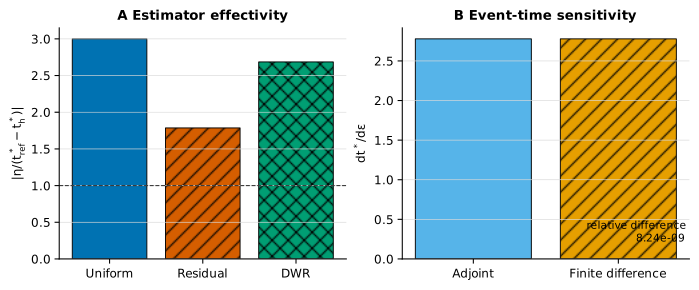
Effectivity 把 estimated signed error $\eta$ 與 $t^*_{ref}-t^*_h$ 比較，理想值接近一。取 absolute value 後，uniform 是 $3.000$ 、residual 是 $1.786$ 、DWR 是 $2.686$ 。預定 smoke band 很寬，為 $[0.1,10]$ ，所以 DWR 沒有在這項失敗；但數值仍未接近到可以支持 calibrated stopping rule。

Derivative verification 是必要而不充分的。它說明 reference event 附近的 endpoint linearisation 對受控 perturbation 表現正確，但不保證 coarse trajectory 已進入 linear regime，也不保證 discrete adjoint 一致表示所有 split operators，或 accumulated residual 已乾淨分離 spatial error。

為何今輪是 uniform 勝出

最直接的線索來自 pilot。24 elements 下，FEM event 是 $53.9806$ ，比 reference 遲約 7.19；first-order DWR correction 是 $-80.336$ ，遠大於真實差距。這顯示 local error representation 被要求在離 reference trajectory 太遠的位置工作。

至少有四個機制值得測試。第一，endpoint 在空間上是 global：cosine coefficients 會積分整個 interval。在低 resolution 下，uniform coverage 可能比 selective mesh 更能保留 global phase balance。第二，indicator 由一個 coarse pilot 凍結；插入新 nodes 後 trajectory 與 adjoint 都會改變，但本次並沒有再次更新 mesh。第三，目前 DWR residual 混合 spatial、temporal、reaction-splitting 與 interpolation effects，而 mesh 只能修正空間部分。第四，相同 production DOF-steps 沒有計算 adaptive overhead。

以上是由 diagnostics 引出的 hypotheses，不是事後選定的結論。它們的用途，是把「DWR 輸了」變成可區分 coarse-linearisation problem、endpoint choice 與 cost accounting 的下一輪實驗。

這個結果能說明甚麼，仍有甚麼未解

結果支持一個有限而清楚的結論：chosen synthetic system 中存在 smooth mode-6 to mode-7 event；independent reference 把它定在 $46.7916$ ；simultaneous refinement 只移動 $0.000641$ ；root 是 transversal；event derivative 與 finite difference 吻合。三個 36-element FEM runs 都找到一個事件。在相同 production DOFs 下，event-time error 由小至大依次是 uniform、DWR、residual。

結果不表示 uniform meshes 一般地較好，也不表示 DWR 不適用於 event time。今次只有一組 parameters、一個 initial perturbation、一個 event、一個 pilot size、一個 production size 與一個 time step。尚未完成 convergence ladder，亦未比較 equal total runtime、分離 estimator 的 space/time contributions、處理二維 geometry、測試 remeshing transfer、擬合 biological data 或跨 seeds 的 robustness。

所以本文的「最好」，只指三個 36-element runs 中 observed absolute event-time error 最小，不是更廣泛的方法排名。

下一步應測試甚麼

下一個實驗應保留今次 smoke result，加入正式 refinement ladder。Pilot 與 production sizes 應在至少三個預定 budgets 中一同增加；每個 budget 都使用同一三種 strategies、independent reference 與 event definition。主要圖表應同時展示 error 對 production work 及 total runtime。

Estimator 亦應分拆 spatial、temporal、reaction 與 splitting contributions。固定 mesh 再縮小 time step，可以檢查 $\Delta t=0.02$ 是否掩蓋 spatial adaptation 的收益。Repeated DWR cycles 可測試 one-shot limitation 是否關鍵。若 coarse pilot 一直不在可靠 linear regime，可考慮 continuation，由較容易的 event approximation 漸進至 registered root。

Robustness 應使用預先指定的 initial spectra，而不是不斷抽 seeds 直到 DWR 勝出。Alternative mode pairs 與 growth-pulse amplitudes 可以在保持 endpoint 可比較的前提下，測試結論是否只來自特殊 phase alignment。若將來要提升 claim，DWR 應在較細 budgets 穩定降低 error、effectivity 趨近一、沒有 missed 或 extra roots，並完整計算 pilot 與 adjoint overhead。

如何把四張圖連起來閱讀

四張圖回答不同問題，而且次序不能倒轉。Reference-event 圖先問 target 是否穩定。若 blue 與 orange crossings 肉眼可見地分開，production methods 的排名便會承接 reference uncertainty。現在兩者幾乎重疊，measured shift 亦很小，表示 target 通過第一關。Nonzero slope 再排除一條幾乎平坦的曲線剛好擦過零點。

Mesh 圖顯示 strategies 真正改變了甚麼。只寫「residual」或「DWR」很容易令人以為 method name 已完整描述 calculation，其實 selected nodes 本身就是結果。Residual mesh 在中段與右半配置較多新增 nodes，其他地方保留較寬 gaps；DWR 則較集中左半，右方出現更闊 elements。兩者使用同一 pilot，卻因 indicators 所問的問題不同而得到不同 placement。

Error 圖才是主要答案。左 panel 比較 registered endpoint，所以 ranking 由它決定；右 panel 是 diagnosis。Uniform 同時有最低 event error 與 field error，而 residual 與 DWR 在兩個 axes 的次序互換。這個互換說明 event functional 確實提供額外資訊：若所有 metrics 永遠產生相同排名，goal-oriented construction 便沒有增加多少理解。

Sensitivity/effectivity 圖把已驗證與仍未解的部分分開。兩條 derivative bars 幾乎完全一致，支持 adjoint terminal condition 所用 calculus；effectivity bars 卻明顯高於一，顯示 coarse resolution 下仍系統性高估 error magnitude。只看 derivative 會過度樂觀，只看 effectivity 又會忽略 endpoint derivative 已通過強獨立核對。

四張圖合起來才是完整 reasoning chain：target 穩定；strategies 真的產生不同 meshes；errors 有清楚排序；estimator 在方向上有資訊，但 calibration 尚未足夠。

公平比較不只看最後 mesh 大小

「相同 elements」只回答一種資源問題。三個 production runs 在同一 time levels 解相同數目的 unknowns，因此 adaptive method 不能單靠較大的 final system 勝出。這令 primary approximation comparison 容易檢查。

可是 residual 與 DWR 需要 uniform 不需要的工作。兩者先解 coarse pilot；residual 再計算及累積 indicators；DWR 還要把 trajectory interpolate 至 enriched space、assemble linearised operators、解 backward adjoint，再把 contributions 投回 parent elements。若 endpoint 是 wall-clock efficiency，這些成本都必須計算。

即使 matrix dimensions 相同，一個 DOF-step 在不同 meshes 上的 hardware cost 亦未必完全相同。Sparse structure、conditioning、cache behaviour 與 solver implementation 都可影響 runtime。今次三個 solve times 相近，但單一 machine 與單次 execution 不足以支持 efficiency claim；應用 repeated timings 與預定 summary statistic。

因此，下一輪應同時報兩種 curves。第一種是 approximation efficiency，即 event error 對 primal DOF-steps，用來隔離 forward mesh placement 的作用。第二種是 end-to-end efficiency，即 event error 對包含 pilot、estimator、adjoint、transfer 與 rejected cycles 的 total cost。DWR 可能在第一種改善而在第二種輸掉，亦可能相反；兩種答案都有研究價值。

Stopping rule 亦涉及公平。若 uniform 固定 36 elements，而 DWR 可一直 refine 至 estimator tolerance，兩者便不再共享 budget；若全部強行停在同一 element count，又可能阻止 estimator 進入可靠 regime。Refinement ladder 可以把單點勝負改成 curve comparison：不只問「36 elements 誰勝」，而是問 error 下降速度及其 total cost。

負面的 adaptive result 為何有用

Computational method 的故事有時由成功的最後一張圖倒推：調整 parameters、挑一個好看的 adaptive mesh，再把最佳例子放在 headline。這會令讀者難以分辨 robust advantage 與看過結果後的 selection。今次預先固定 error ceiling 與 decision rule，正正令不方便的答案能夠保留下來。

這次失敗比「resolution 不足」提供更多資訊。三種 meshes 使用同一 resolution，errors 卻有系統差異；三者都找到相同類型 crossing，所以不是 missed-event convention；reference uncertainty 太小，無法解釋 ranking；event derivative 又已 verification，所以基本 sign 或 denominator mistake 亦不大可能。剩下的 hypotheses 已收窄至 pilot quality、residual decomposition、global phase representation 與 repeated adaptation。

結果亦阻止兩種容易但誤導的替代說法。因為 DWR 在 event time 勝過 residual，不能就此宣布 goal orientation 已成功；因為 uniform 最好，也不能宣布 adaptivity 有害。Observed order 是真實結果，但所有 methods 都未通過 absolute accuracy condition。正確結論是 Phase 1 得到 diagnostic ordering，尚未得到 successful approximation。

這與實驗科學的 acceptance tolerance 相似：三件 instruments 全部超標時，bias 最小的一件不會自動取得 certification。它的相對優勢可以指引 redesign，但仍須通過 absolute criterion。Numerical research 也需要同樣紀律。

負結果在保留可改進 machinery 時尤其有價值。Independent reference、modal event、matched meshes、sensitivity check、estimator output 與 visual diagnostics 已形成 reusable baseline。下一輪可以每次只改一個 axis，再與保留的 smoke result 比較，而不是靜靜替換 coarse configuration，只展示後來成功的版本。

保護結論的核對

不同 checks 保護不同 interpretation。Reference refinement 保護所有 event errors 的 denominator；transversality 保護 root 的 local stability；adjoint 對 finite difference 保護 event derivative；equal production DOF-steps 保護主要 resource comparison；final-field error 防止 event metric 隱藏廣泛 state degradation；effectivity 則揭示 estimator 是否 calibrated，而不只是能輸出有限數字。

Software tests 的角色較窄。它們檢查 matrix symmetry、conservation-related properties、modal projection、event location、mesh splitting、configuration loading、sensitivity agreement 與 smoke pipeline。通過 tests 不會驗證 Schnakenberg model，更不會證明 DWR theorem；它只表示 reported calculation 能抵受常見 coding failures 的針對性檢查。

Visual quality 同樣影響解讀。Colours 同時配合 markers 或 hatching，避免只靠 hue 區分 strategies；axes 寫出真正 error quantities，而非含糊的 performance scores；reference plot 明確說明 local linearisation；captions 亦交代 cost comparison 不包含 overhead。這些做法不改變 data，卻減少讀者推論超出實驗範圍。

最重要的保護仍是 claim boundary：這是一個 deterministic one-shot Phase 1 smoke experiment。它的任務是判斷目前設計是否值得直接擴大，以及指出下一步要改甚麼。按這個標準，它已完成工作：拒絕即時 promotion，並給出集中而可測試的下一輪計劃。

Event-driven modelling 的實際工作次序

這個 workflow 不只適用於今次 PDE。第一步應把 event 寫成 scalar mathematical condition，清楚包括 crossing direction、earliest admissible time，以及有多個 roots 時的選擇規則。若只寫「pattern 改變的時間」，不同研究者可以用 peak count、modal dominance、threshold 或目測圖像得到不同答案。先定義 endpoint，才知道 error 的 denominator 究竟是甚麼。

第二步是建立 uncertainty 足夠小的 independent reference。Reference 並不需要聲稱 exact solution，但 refinement shift 必須遠小於 methods 之間想比較的差距。今次 $0.000641$ 與 production errors 的比例足以支持 ranking；若兩者同一量級，圖中的 bar order 便沒有解釋力。Reference solver 採用另一 spatial representation，亦可以減少同一 assembly mistake 同時污染 benchmark 與 competitors 的風險。

第三步是檢查 transversality。當 $\dot G(t^*)$ 接近零，極小 field perturbation 都可造成很大的 time shift，甚至把一個 root 變成兩個或完全消失。在這種情況下，event-time accuracy 可能主要反映 root conditioning，而非 mesh quality。將 slope 與 refinement shift 一起報告，比只列出一個看來很精確的 $t^*$ 更誠實。

第四步才是讓 adaptive indicator 接受測試。Pilot 不應只被視為產生 mesh 的內部步驟，它本身也需要 acceptance check。應比較 pilot event 與 reference，並檢視 predicted correction 的 scale。若 correction 比 observed discrepancy 大許多，這不是單純「數值不漂亮」，而是 linearisation-based marking 可能已離開 useful regime 的證據。合理回應可以是增加 pilot resolution、獨立縮小 time step、重複 adaptation，或先分解 residual，而不是直接擴大 production run。

最後，應同時保留 target metric 與 broad state metric。前者回答真正科學問題，後者檢查為了優化 endpoint 是否令其餘 solution 大幅惡化。兩者不能偷偷互換：field error 較小不代表 event time 較準，event time 偶然準確亦不表示整個 trajectory 已可靠。這種雙重視角令 preferred method 即使沒有勝出，計算仍然可解讀。

若把問題帶到二維會改變甚麼

一維 reference interval 令 cosine modes、node placement 與 no-flux boundaries 都相對清楚。若擴展至二維 growing surface 或 tissue-like domain，難度不只來自 DOFs 增加。Domain mapping 可能產生 anisotropic metric terms，mesh quality 會受 deformation 影響，而 pattern identity 亦未必能由單一 mode pair 描述。

在二維，事件可以是 spectral subspace 之間的 energy crossing、某個 connected component 首次形成，或者 geometric interface 到達指定位置。後兩者往往 nonsmooth，可能需要 regularisation 或不同 goal functional。若 event definition 改變，adjoint terminal condition、transversality check 與 reference strategy 都要重新推導，不能直接搬用今次一維公式。

Mesh adaptation 亦需要同時處理 geometry 與 solution。Element refinement 可降低 spatial approximation error，但 domain movement 可能造成 skewness；remeshing 又引入 field-transfer error。若只計算 primal DOF-steps，便可能完全漏掉 mesh generation 與 transfer cost。二維 study 因此更需要把 approximation efficiency 與 end-to-end efficiency 分開報告。

這些困難不表示二維工作不值得做，而是說 Phase 1 的用途正是先在最清楚環境中暴露 estimator mechanism。只有當 refinement ladder 顯示 event-time error 隨 resolution 有可理解趨勢，才值得把 geometry、topology 與 remeshing uncertainty 同時加入。

對結果展示的最後一項要求

科學圖表不只是裝飾。若 bar chart 使用含糊的 normalized score，讀者無法知道差異是否超出 reference uncertainty；若三種策略只靠顏色區分，色覺差異或黑白列印會破壞信息；若 caption 不說明 matched work 是否包含 adjoint overhead，公平性便容易被誤讀。

因此今次 figures 採用直接 quantity labels、colour 加 marker 或 hatching，以及簡短但具體 captions。Reference panel 把 tiny shift 與 slope 放在同一畫面；mesh panel 顯示實際 node locations；strategy panel 把主要 event error 與 secondary field error 分開；verification panel 則把 derivative agreement 與 estimator calibration 並列。四張圖在原尺寸及 Blog layout 都要檢查 labels、legend、caption 與相鄰內容是否 overlap 或 clipping。

這種視覺 QA 不會令弱證據變強，但可以避免強證據因排版而被誤讀。對一篇以方法失敗機制為主線的文章尤其重要：圖必須讓讀者看到失敗發生在哪一層，而不是用設計效果把它掩蓋。

為何不應只報最好的一個數字

若文章只列出 uniform 的 $2.6001$ ，讀者不知道它與其他 strategies 的距離，也不知道這個數字是否已通過 accuracy target。若只報三個 errors 而省略 reference shift，讀者又無法判斷差異是否大過 benchmark uncertainty。若只報 ranking 而不報 pilot，則最有用的 failure clue 會消失。因此每一個主要數字都需要一個比較對象：production error 對 reference uncertainty、DWR estimate 對 observed error、event metric 對 field metric、primal work 對 total overhead。

同一道理適用於文字結論。寫「uniform wins」必須緊接限定語，說明只是在這三個 36-element runs 中 observed error 最小。寫「DWR estimator passes」也要說明通過的是很寬的 smoke band，而 effectivity 並未接近一。寫「sensitivity verifies」則要分清楚，它驗證的是 local event derivative，不是整套 adaptive workflow。

這些限定不是削弱文章，而是令結果可以累積。當 refinement ladder 完成後，新數據可直接回答目前未解的問題：uniform advantage 是否隨 budget 消失、effectivity 是否向一收斂、pilot correction 是否回到合理 scale，以及 DWR overhead 是否換來足夠 accuracy。若今次只留下一句勝負，下一輪就沒有清楚 baseline 可比較。

一個可被推翻的下一輪預測

現有 diagnostics 支持一個可測試預測：若主要問題真是 coarse pilot 離 reference 太遠，增加 pilot resolution 或加入第二個 DWR cycle 後，correction magnitude 應明顯下降，effectivity 應靠近一，而 DWR event-time error 相對 uniform 應改善。這三項必須一起觀察；只看到 mesh 變得更集中，並不足以確認機制。

相反，若 pilot 改善後 uniform 仍穩定最好，而 spatial residual contribution 已能與 time/splitting terms 分開，便可能表示 global modal endpoint 在此 regime 本來就較受惠於均勻 phase coverage。那會是一個比「adaptive method 沒用」精確得多的結論，也能指導何時選擇 goal-oriented mesh、何時保留 uniform baseline。

若縮小 time step 後三者 errors 同步大幅下降，則現時 spatial ranking 可能被 temporal error 污染。若 ranking 對 initial spectra 很敏感，則應報 distribution 或 regime map，而非單一 seed 的 winner。每種可能結果都對應不同 mechanism，這正是預先寫清楚 predictions 的好處。

從 smoke test 到可支持結論的距離

Smoke test 的價值是快速暴露設計問題，不是以最小計算量換取最大 claim。今次已確認 event 存在、reference 足夠穩定、三種 meshes 能在相同 production size 下完成，以及 estimator 可以輸出有符號 correction。這些是進入正式 convergence study 的必要條件，但不是完成條件。

要把結論提升，至少需要三個互相配合的趨勢。第一，隨 production budget 增加，各 methods 的 event-time error 應一致下降，而非在某一點偶然交叉。第二，reference refinement 要比最細 production error 更嚴格，否則 convergence curve 尾端只是在量度 benchmark noise。第三，effectivity 應逐步靠近一；若 accuracy 改善但 estimator calibration 不改善，就不能用它作 reliable stopping criterion。

還要避免把同一份 pilot data 同時用作設計、選擇與最終評估。Pilot 可以幫助決定 refinement strategy，但 promotion 應在預先固定的新 budgets 或新 initial spectra 上驗證。若每次看完 ranking 才改 mesh rules，再把最好一次稱為 final，method comparison 就會混入 selection bias。

文章因此保留 REFRAME 這個一次性的研究狀態，但沒有把它變成整篇的管理語言。對讀者而言，最重要的是實際結果與原因：uniform 在 36 elements 下最準，DWR 排第二，三者都未達標，而 coarse pilot 提供下一步最值得測試的解釋。這些資訊已足以形成一篇完整研究故事，同時沒有把尚未完成的 convergence evidence 寫成既定事實。

這亦解釋為何今次不把 runtime 的偶然先後寫成 performance ranking。單次 execution 會受 operating-system scheduling、cache state 與背景工作影響；真正 wall-clock comparison 應固定環境、warm-up 規則及 repetition count，再以 median 或預定 statistic 報告。現階段使用 primal DOF-steps，只能回答相同 forward resolution 下的 approximation question。把這個界線說清楚，才不會令讀者誤以為圖中的 accuracy order 同時也是 speed order。

同時，未來若改動 indicator 或 pilot size，應保留今次 configuration 作為 baseline，而不是覆寫原有數字。只有並列新舊結果，才能知道改善來自 resolution、重複 adaptation、較細 time step，還是純粹換了較有利的 initial condition。這種版本化比較亦可防止 negative result 在後續成功後消失。對研究讀者而言，方法如何由失敗走向可靠，往往比一張最後勝出的圖更有參考價值。

換句話說，下一輪不應以「找一個 DWR 勝出的例子」為目標，而應以「找出哪個誤差機制控制 ranking」為目標。前者只需要搜索 parameters，後者卻需要對照實驗、分解 estimator 並保留失敗個案。只有後者才能產生可轉移到其他 event-driven PDE problems 的知識。

這亦是本文保留完整限制與下一步設計的原因：讀者不只看到誰勝誰負，也能判斷現有證據距離可推廣結論尚有多遠。

這個距離本身也是結果。

結論

這個 Phase 1 終於完成標題所問的 mesh comparison，而答案是有條件的：mesh 可以保留事件，但在這個 coarse matched budget 下，獲得最多目標資訊的 mesh 並沒有保留得最好。

Reference 足以支持比較：transition 是 $46.7916$ ，refinement shift 只有 $0.000641$ ，crossing 是 transversal，adjoint derivative 與 finite difference 相符。Production result 亦很清楚：uniform error 是 $2.6001$ 、DWR 是 $3.2752$ 、residual 是 $4.4030$ 。全部超過 registered ceiling，所以 verdict 是 REFRAME。

這個結果比勉強宣稱成功更有價值。它指出 late pilot、oversized DWR correction、global modal endpoint 與 mixed residual contributions 都是下一輪的具體測試目標。下一個 claim 必須來自 refinement ladder，而不是重新命名今次 smoke run。

參考文獻

Crampin, Gaffney, and Maini, “Reaction and Diffusion on Growing Domains” (1999), DOI 10.1006/bulm.1999.0131。
Crampin, Gaffney, and Maini, “Mode-Doubling and Tripling in Reaction-Diffusion Patterns on Growing Domains” (2002), DOI 10.1007/s002850100112。
Madzvamuse, Wathen, and Maini, “A Moving Grid Finite Element Method Applied to a Model Biological Pattern Generator” (2003), DOI 10.1016/S0021-9991(03)00294-8。
Madzvamuse and Maini, “Velocity-Induced Numerical Solutions of Reaction-Diffusion Systems on Continuously Growing Domains” (2007), DOI 10.1016/j.jcp.2006.11.022。
MacKenzie and Madzvamuse, “Analysis of Stability and Convergence of Finite-Difference Methods for a Reaction-Diffusion Problem on a One-Dimensional Growing Domain” (2011), DOI 10.1093/imanum/drp030。
Lakkis, Madzvamuse, and Venkataraman, “Implicit-Explicit Timestepping with Finite Element Approximation of Reaction-Diffusion Systems on Evolving Domains” (2013), DOI 10.1137/120880112。
Venkataraman, Lakkis, and Madzvamuse, “Adaptive Finite Elements for Semilinear Reaction-Diffusion Systems on Growing Domains” (2013), DOI 10.1007/978-3-642-33134-3_8。
Xie and Hu, “Finite Element Simulations with Adaptively Moving Mesh for the Reaction Diffusion System” (2016), DOI 10.4208/nmtma.2016.m1229。
Chaudhry, Estep, Stevens, and Tavener, “Error Estimation and Uncertainty Quantification for First Time to a Threshold Value” (2021), DOI 10.1007/s10543-020-00825-0。
Li and Yi, “A Posteriori Error Estimates of Goal-Oriented Adaptive Finite Element Methods for Nonlinear Reaction-Diffusion Problems” (2022), DOI 10.1016/j.cam.2022.114362。
Chaudhry 等, “Error Estimation for the Time to a Threshold Value in Evolutionary Partial Differential Equations” (2023), DOI 10.1007/s10543-023-00947-1。
Endtmayer, Langer, and Schafelner, “Goal-Oriented Adaptive Space-Time Finite Element Methods for Regularized Parabolic p-Laplace Problems” (2024), DOI 10.1016/j.camwa.2024.05.017。