
The most interesting result of this experiment is the one I did not expect: giving a mesh more information did not make it more accurate. With the same 36-element production budget, a uniform finite-element mesh located the modal transition more accurately than either a conventional residual mesh or a dual-weighted-residual (DWR) mesh designed for that event.
The independent spectral reference placed the transition at . The uniform mesh reported , an absolute error of . DWR reduced the error relative to residual adaptation, but still arrived at , or late. The residual mesh was last at , or late. All three missed a registered accuracy ceiling of 1.5 time units, so the Phase 1 verdict is REFRAME, not a claim that uniform refinement is generally superior.
That distinction matters. DWR is not disproved by one coarse, one-shot trial. Instead, the experiment exposes a concrete failure mechanism: the adaptive meshes were selected from a 24-element pilot whose own event was already about 7.19 time units late. Its first-order DWR correction was also extremely large. A mesh indicator built around that poor linearisation can emphasize mathematically relevant locations and still fail to repair the event time.
What the experiment found
| Question | Finding | Why it matters |
|---|---|---|
| Is there a stable reference event? | The comparison has a defined target. | |
| Does reference refinement move it? | time units | Reference uncertainty is tiny beside every FEM error. |
| Is the crossing transversal? | The root is not nearly tangent. | |
| Which mesh is best at 36 elements? | Uniform, error | Selective placement did not win this smoke test. |
| How did DWR perform? | Error , effectivity | It ranked second and overestimated the error magnitude. |
| How did residual adaptation perform? | Error | Reducing a field residual did not protect the event. |
| Did any FEM run pass the error ceiling? | No | The next step is a refinement ladder, not promotion. |
The experiment is deliberately small. It establishes that the reference, event derivative, three equal-size production meshes, and error estimator can all be executed coherently. It does not establish an asymptotic rate, a cost advantage, or a universal ranking.
Why the question is about an event, not a field
Reaction–diffusion simulations produce concentrations over space and time. The scientific statement of interest may instead concern when the field changes character. A tissue pattern may gain a stripe, a chemical mode may overtake another mode, or an activation front may first reach a threshold. These are event questions.
Field accuracy and event accuracy are related but not interchangeable. A solution can have a modest norm error while moving a threshold crossing appreciably. Conversely, a field may differ away from the critical modes but preserve their crossing time. If the question is “when?”, refining a mesh solely where the field residual is large may spend resolution in the wrong place.
This study uses a modal transition because it is smoother than peak counting. Let denote the cosine coefficient of the activator perturbation for mode . The event functional is
The event time is the first negative-to-positive root after :
Before the crossing, mode 6 carries more squared amplitude; afterwards, mode 7 does. Squaring avoids an arbitrary modal sign, and a transversal crossing gives a differentiable local event time. The definition measures a precise transfer of spectral dominance. It should not be silently re-described as a topological split or a biological developmental landmark.
Peak count was excluded. Counting maxima looks intuitive, but it is discontinuous under small perturbations, depends on prominence and smoothing rules, and can change when a shallow shoulder appears. A modal equality provides a clean scalar root for verification and adjoint analysis.
The growing-domain model
The benchmark is a one-dimensional Schnakenberg reaction–diffusion system on a prescribed growing interval. After mapping the physical coordinate to a fixed reference coordinate , the concentrations satisfy
with no-flux conditions. Here , , , and . The domain has a slow exponential component and a smooth growth pulse centred near . As changes, diffusion weakens in reference coordinates and the dilution term removes concentration at rate .
This combines two mechanisms. Reaction and diffusion determine which modes can grow, while domain growth changes physical wavelengths and the effective diffusion scale. The pulse makes the mode-6 to mode-7 passage occur within 60 time units. The initial perturbation contains several cosine components and uses a fixed seed. None of these choices represents fitted biological data.
The reference coordinate lets every mesh occupy the same unit interval. A node at moves physically as changes, but its reference label remains fixed. The comparison can therefore separate element placement from physical expansion.
Why earlier work narrowed the contribution
Growing-domain pattern formation is established. Crampin, Gaffney, and Maini derived reaction–diffusion equations on growing domains and studied frequency-doubling in the Schnakenberg system. Later studies developed moving-grid and evolving-domain schemes, analysed convergence, and showed that grid motion can affect selected patterns. The facts that growth can alter a Turing pattern and that finite elements can simulate it are not new contributions here.
Adaptivity is also prior art. Residual estimators for semilinear reaction–diffusion systems and adaptive finite elements on growing domains already exist. Goal-oriented methods weight residuals with an adjoint associated with a chosen quantity. First-time-to-threshold functionals have their own error-representation literature because moving a root is not the same problem as reducing a state norm.
The useful gap is narrower: take one smooth event, verify an independent reference, give uniform, residual, and DWR strategies the same production degrees of freedom, and retain the result even if the goal-oriented method does not win. This is a benchmark question, not a novelty claim for any ingredient.
Two numerical views of the transition
The reference solver is intentionally different from the compared finite-element solver. It uses cell-centred cosine modes, a fine 512-cell representation, and Strang splitting with a step of . Diffusion is diagonal in cosine space, while reaction and dilution use a second-order update. A simultaneous refinement doubles the cells and halves the time step.
The production solver uses nodal continuous piecewise-linear finite elements. It assembles consistent mass and stiffness matrices on each mesh, advances reaction and dilution at the same temporal order, and treats diffusion with Crank–Nicolson. Its time step is . The event is evaluated through quadrature-based cosine projections.
The solvers share the model, initial state, and event, but not their spatial representation or diffusion update. Agreement addresses a useful class of implementation errors. It cannot rule out an error in assumptions shared by both and does not supply experimental validation.
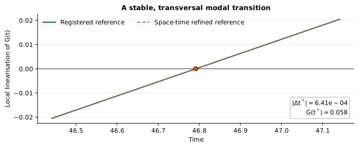
The reference crossing occurs at . Refining space and time moves it to . The shift, , is over four thousand times smaller than the best production error. The crossing slope is , far above the registered floor of . Thus an unresolved or tangent reference root is not deciding the comparison.
Three meshes with one budget
Every production mesh has 36 elements and 37 degrees of freedom per scalar state. With two variables and 3,000 steps, each solve uses 222,000 primal degree-of-freedom steps. This is a matched primal-work proxy, not matched wall-clock cost. The pilot, indicator, enriched adjoint, and mesh selection add overhead to adaptive strategies.
The uniform mesh divides the interval equally. The residual mesh starts from a 24-element pilot, accumulates flux-jump indicators for both fields, and splits the largest-scoring elements. The DWR mesh solves an enriched backward adjoint whose terminal condition comes from event-time sensitivity. It weights the residual by that adjoint up to the pilot event, then refines the largest contributors.
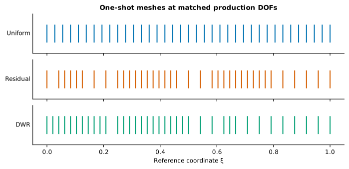
These are one-shot designs, not repeated solve-estimate-mark-refine cycles. This limitation is central. A goal-oriented method depends on a useful primal and adjoint linearisation; one coarse pilot may be too inaccurate for its indicator to predict what a later mesh needs.
The matched-work result
The uniform mesh is best on both reported errors. Its event time of is late, and its relative final-field error is . DWR gives , late, with field error . Residual adaptation gives , late, with field error .
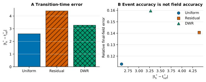
Adaptivity is not automatically advantageous at a fixed coarse budget. Uniform coverage can protect global phase balance for a cosine functional. The adaptive rankings also depend on the endpoint: DWR is worse than residual on field error but better on event time, consistent with its goal even though it does not beat uniform.
No run misses the event. The failure is quantitative: every event appears, but every FEM time is more than 1.5 units from the reference. That ceiling was fixed before reading the ranking. Phase 1 therefore calls for diagnosis, not promotion of the least inaccurate method.
What the adjoint checks
For a transversal root , a perturbation changes the event time to first order by
This supplies the terminal quantity for the backward adjoint and a direct verification target. The analytic event-time derivative is for a declared modal perturbation. A centred finite difference gives . Their relative difference is .
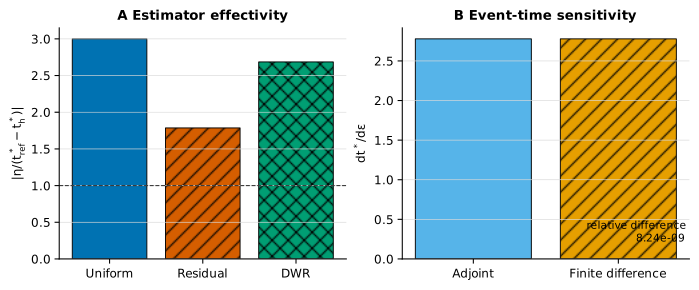
Effectivity compares an estimated signed error with . A value near one is ideal. Absolute effectivities are for uniform, for residual, and for DWR. The registered smoke band was broad, , so DWR does not fail it. Yet none is close enough to one for a calibrated stopping rule.
Derivative verification is necessary but insufficient. It shows that endpoint linearisation behaves under a controlled perturbation near the reference. It does not guarantee that a coarse trajectory lies in the linear regime, that a discrete adjoint represents every split operator, or that an accumulated residual isolates spatial error.
Why uniform won this round
The immediate clue is the pilot. On 24 elements, the FEM event occurs at , about 7.19 units after the reference. The first-order DWR correction is , far larger than the true discrepancy. The local representation is being asked to operate too far from the reference trajectory.
Four mechanisms deserve testing. First, the endpoint is global: cosine coefficients integrate over the whole domain. Uniform coverage may preserve global phase balance better than selective refinement at low resolution. Second, the indicator is frozen from one coarse pilot; after inserting nodes, the trajectory and adjoint change but the mesh is not updated again. Third, the current residual mixes spatial, temporal, reaction-splitting, and interpolation effects, although the mesh can act only on space. Fourth, equal production DOF-steps exclude adaptive overhead.
These are hypotheses, not post hoc conclusions. Their value is to turn “DWR lost” into experiments that can distinguish a coarse-linearisation problem from an unsuitable endpoint or an accounting problem.
What this result does, and does not, show
The result supports a limited statement. A smooth mode-6 to mode-7 event exists. An independent reference resolves it at ; simultaneous refinement moves it only ; the root is transversal; and the event derivative matches finite differences. All three 36-element FEM runs detect one event. At equal production degrees of freedom, uniform has the smallest event-time error, followed by DWR and residual.
It does not show that uniform meshes are generally better or that DWR is unsuitable for event times. There is one parameter set, initial perturbation, event, pilot size, production size, and time step. No convergence ladder is complete. The study does not compare equal total runtime, separate spatial from temporal estimator contributions, treat two-dimensional geometry, test remeshing transfer, fit biological data, or sample robustness over seeds.
Here “best” means only the smallest observed event-time error among these three 36-element runs. It is not a ranking beyond them.
What should be tested next
The next experiment should preserve this smoke result and add a refinement ladder. Pilot and production sizes should increase together across at least three registered budgets. Each budget should include the same three strategies, independent reference, and event. The main comparison should show error against both production work and total runtime.
The estimator should separate spatial, temporal, reaction, and splitting terms. Time-step refinement at fixed mesh would reveal whether masks spatial gains. Repeated DWR cycles would test the one-shot limitation. If the pilot remains outside the useful linear regime, continuation could move from an easier approximation toward the registered root.
Robustness should use a preregistered set of initial spectra, not repeated draws until DWR wins. Alternative mode pairs and pulse amplitudes can test how global the result is while keeping the endpoint comparable. Promotion should require stable improvement at finer budgets, effectivity approaching one, no missed or extra roots, and transparent pilot and adjoint overhead.
How to read the four figures together
Each figure answers a different question, and their order matters. The reference-event panel asks whether there is a sufficiently stable target. If the blue and orange crossings were visibly separated, any ranking of the production methods would inherit that ambiguity. They are almost coincident, and the measured shift is tiny, so the target passes this first check. The nonzero slope adds another safeguard: the event is not created by a flat curve grazing zero.
The mesh panel then shows what the strategies actually changed. It is tempting to describe an adaptive method only by its name, as though “residual” or “DWR” uniquely determined a computation. In practice, the selected nodes are part of the result. The residual mesh spends many of its added nodes around the centre and right half, with several coarse gaps elsewhere. DWR concentrates more strongly in the left half and leaves visibly wider elements toward the right. Those choices reflect different accumulated indicators from the same pilot.
The error panel is the experiment’s answer. Its left side compares the registered quantity, so that side determines the ranking. The scatter on the right is diagnostic. Uniform lies at the lowest event error and lowest final-field error. Residual and DWR swap order across the two axes. That swap is evidence that the event functional is doing real work: had every method ranked identically under every metric, the goal-oriented construction would have added little information.
Finally, the sensitivity and effectivity panel separates a verified component from an unsettled one. The two derivative bars agree almost perfectly, supporting the calculus used to construct the adjoint terminal condition. The effectivity bars are not as reassuring. They sit above one, showing systematic overprediction of error magnitude at this resolution. Reading only the derivative panel would therefore be too optimistic; reading only the effectivity panel would obscure that the endpoint derivative itself has passed a strong independent check.
Together the figures form a chain: the target is stable, the strategies make materially different meshes, the resulting errors have a clear ordering, and the estimator is directionally useful but poorly calibrated. No single panel carries the whole conclusion.
Fairness is more than matching the last mesh
“Same number of elements” sounds like an unambiguous fairness condition, but it answers only one accounting question. All three production runs solve the same number of unknowns at each of the same time levels. This prevents an adaptive method from winning merely by using a larger final system. It also makes the primary comparison easy to inspect.
However, residual and DWR need information that uniform refinement does not. Both first solve the coarse pilot. Residual then calculates and accumulates indicators. DWR additionally interpolates the trajectory to an enriched space, assembles linearised operators, solves a backward adjoint, and projects contributions back to parent elements. If wall time were the endpoint, those costs would belong in the numerator.
There is another subtlety. A production DOF-step is not identical across meshes at the hardware level. Sparse-matrix structure, conditioning, cache behaviour, and solver implementation can change runtime even when matrix dimensions match. The recorded solve times are close, but one machine and one execution are not enough to make an efficiency claim. Runtime noise should be measured with repetitions and a declared summary statistic.
A future paper should therefore report two comparisons. The first is approximation efficiency: event error against primal DOF-steps, which isolates what a chosen mesh does for the forward solve. The second is end-to-end efficiency: event error against total elapsed cost, including pilot, estimator, adjoint, transfer, and any rejected refinement cycle. DWR could improve the first while losing the second, or vice versa. Both outcomes are scientifically meaningful.
Fairness also applies to stopping rules. If uniform uses 36 elements while DWR is allowed to refine until its estimator is satisfied, the final meshes no longer share a budget. Conversely, stopping every method at the same element count may prevent an estimator from reaching the regime where it becomes reliable. A refinement ladder resolves this tension by comparing curves rather than one selected point. The question becomes not “who won at 36?” alone, but “how rapidly does each error fall, and at what total cost?”
Why a negative adaptive result is informative
Computational method stories are often narrated from a successful final figure backwards. Parameters are tuned, an adaptive mesh looks plausible, and the best example becomes the headline. That workflow makes it hard to distinguish a robust advantage from selection after inspection. Here the error ceiling and decision rule make the inconvenient outcome visible.
The failure contains more information than a generic statement that resolution was insufficient. Uniform, residual, and DWR all use the same resolution, yet their errors differ systematically. All three detect the same type of crossing, so the problem is not a missed-event convention. The reference uncertainty is negligible, so it is not responsible for the ranking. The event derivative verifies, so a basic sign or denominator error is unlikely. What remains is a narrower collection of possibilities involving pilot quality, residual decomposition, global phase representation, and repeated adaptation.
The result also prevents an easy but misleading substitution. Because DWR ranks better than residual on event time, one might announce that goal orientation helps. Because uniform ranks best, one might announce that adaptation hurts. Neither statement is supported. The observed order is real, but the registered accuracy condition fails for all methods. The appropriate conclusion is that Phase 1 has produced a diagnostic ordering without a successful approximation.
This distinction mirrors experimental science. If three instruments all lie outside an acceptance tolerance, the least biased instrument is not automatically certified. Its relative advantage can guide redesign, but certification requires meeting the absolute criterion. Numerical research benefits from the same discipline.
Negative results are especially useful when they preserve the machinery needed to improve. The independent reference, modal event, matched meshes, sensitivity test, estimator output, and visual diagnostics now form a reusable baseline. A refined experiment can change one axis at a time and compare against the retained smoke result. That is much more informative than silently replacing the coarse configuration and presenting only a later success.
Checks that protect the interpretation
Several checks guard different parts of the conclusion. The reference refinement protects the denominator of every reported event error. Transversality protects the local stability of the root. The adjoint-versus-finite-difference comparison protects the event derivative. Equal production DOF-steps protect the primary resource comparison. Recording final-field error prevents the event metric from hiding broad degradation of the state. Reporting effectivity exposes whether the estimator is calibrated rather than merely finite.
Software checks serve a narrower role. The automated tests cover matrix symmetry and conservation-related properties, modal projection, event location, mesh splitting, configuration loading, sensitivity agreement, and the smoke pipeline. Passing them does not validate the Schnakenberg model or prove a theorem about DWR. It shows that the reported calculation survives checks aimed at common coding failures.
Visual quality is also part of interpretation. Colours are paired with markers or hatching, so the strategies remain distinguishable without relying on hue. Axes state the actual error quantities rather than vague “performance” scores. The reference plot labels its local linearisation explicitly. Captions say when a cost comparison excludes overhead. These choices do not change the data, but they reduce the chance that a reader infers more than the experiment measured.
The strongest protection is still the boundary on the claim. This is a deterministic one-shot Phase 1 smoke experiment. Its role is to decide whether the current design deserves a larger study and to reveal what must change. On that standard it succeeds: it rejects immediate promotion and gives a focused plan for the next computation.
A practical lesson for event-driven modelling
The workflow generalises beyond this particular PDE. Begin by writing the event as a scalar mathematical condition, including direction, earliest admissible time, and the rule for multiple roots. Then establish a reference whose uncertainty is small relative to the differences one hopes to compare. Check transversality because a nearly tangent root can turn tiny field errors into unstable time shifts. Only after those steps should an adaptive indicator be judged by event-time error.
This ordering prevents an attractive mesh picture from becoming evidence before the endpoint itself is trustworthy. It also makes failed stages informative rather than embarrassing.
The pilot deserves its own acceptance test. Before using its adjoint to move a mesh, compare its event with the reference and inspect the scale of its predicted correction. A correction vastly larger than the observed discrepancy is not merely an unattractive number; it is evidence that linearisation-based marking may be outside its useful regime. The response need not be to abandon DWR. One can increase pilot resolution, refine time independently, repeat adaptation, or decompose the residual before spending a larger production budget.
Finally, retain two views of quality. The target metric answers the scientific question, while a broad state metric checks that optimizing the target has not damaged everything else. Neither should silently replace the other. This discipline keeps an event-driven computation interpretable even when the preferred method fails to win.
Conclusion
This Phase 1 experiment reaches the comparison implied by its title, and the answer is conditional. A mesh can preserve the event, but the most informed mesh did not preserve it best at this coarse matched budget.
The reference is strong enough: the transition is , refinement changes it by , the crossing is transversal, and the adjoint derivative matches finite differences. The production result is clear: uniform error is , DWR error , and residual error . Every value exceeds the registered ceiling, so the verdict is REFRAME.
That outcome is more useful than a forced success. It identifies a late pilot, oversized DWR correction, global endpoint, and mixed residual contributions as targets. The next claim must come from a refinement ladder, not from relabelling this smoke run.
References
- Crampin, Gaffney, and Maini, “Reaction and Diffusion on Growing Domains” (1999), DOI 10.1006/bulm.1999.0131.
- Crampin, Gaffney, and Maini, “Mode-Doubling and Tripling in Reaction-Diffusion Patterns on Growing Domains” (2002), DOI 10.1007/s002850100112.
- Madzvamuse, Wathen, and Maini, “A Moving Grid Finite Element Method Applied to a Model Biological Pattern Generator” (2003), DOI 10.1016/S0021-9991(03)00294-8.
- Madzvamuse and Maini, “Velocity-Induced Numerical Solutions of Reaction-Diffusion Systems on Continuously Growing Domains” (2007), DOI 10.1016/j.jcp.2006.11.022.
- MacKenzie and Madzvamuse, “Analysis of Stability and Convergence of Finite-Difference Methods for a Reaction-Diffusion Problem on a One-Dimensional Growing Domain” (2011), DOI 10.1093/imanum/drp030.
- Lakkis, Madzvamuse, and Venkataraman, “Implicit-Explicit Timestepping with Finite Element Approximation of Reaction-Diffusion Systems on Evolving Domains” (2013), DOI 10.1137/120880112.
- Venkataraman, Lakkis, and Madzvamuse, “Adaptive Finite Elements for Semilinear Reaction-Diffusion Systems on Growing Domains” (2013), DOI 10.1007/978-3-642-33134-3_8.
- Xie and Hu, “Finite Element Simulations with Adaptively Moving Mesh for the Reaction Diffusion System” (2016), DOI 10.4208/nmtma.2016.m1229.
- Chaudhry, Estep, Stevens, and Tavener, “Error Estimation and Uncertainty Quantification for First Time to a Threshold Value” (2021), DOI 10.1007/s10543-020-00825-0.
- Li and Yi, “A Posteriori Error Estimates of Goal-Oriented Adaptive Finite Element Methods for Nonlinear Reaction-Diffusion Problems” (2022), DOI 10.1016/j.cam.2022.114362.
- Chaudhry and colleagues, “Error Estimation for the Time to a Threshold Value in Evolutionary Partial Differential Equations” (2023), DOI 10.1007/s10543-023-00947-1.
- Endtmayer, Langer, and Schafelner, “Goal-Oriented Adaptive Space-Time Finite Element Methods for Regularized Parabolic p-Laplace Problems” (2024), DOI 10.1016/j.camwa.2024.05.017.