How Noise Flips a Genetic Switch

A deterministic genetic switch can have two stable states. Once an ordinary differential equation enters one basin of attraction, it remains there unless an external perturbation crosses the separatrix.

A cell does not evolve as a smooth concentration field. Molecules are counted in finite numbers; production and degradation events occur one at a time. A sequence of individually ordinary reaction events can occasionally push the circuit across a deterministic basin boundary.

This study places those two descriptions side by side. An ODE reveals the geometry of bistability. An exact-event Gillespie simulation reveals how molecular system size controls spontaneous switching, memory lifetime, stationary probability, and the success of an induction pulse.

The model is synthetic. It is inspired by the mutually repressing toggle architecture, not calibrated to a particular organism or plasmid.

Deterministic memory

Let (u) and (v) be concentrations of two proteins that repress each other:

\frac{du}{dt} =\frac{\alpha_u}{1+v^{n_v}}-\delta_u u,

\frac{dv}{dt} =\frac{\alpha_v}{1+u^{n_u}}-\delta_v v.

The symmetric default parameters are

\alpha_u=\alpha_v=3,\qquad n_u=n_v=2,\qquad \delta_u=\delta_v=1.

Each nullcline states where one protein’s production equals its degradation. Their intersections are equilibria. Numerical root finding from a grid of initial guesses finds three:

(u,v)\approx(2.618,0.382),\quad(1,1),\quad(0.382,2.618).

Jacobian eigenvalues classify the two asymmetric equilibria as stable and the central symmetric equilibrium as a saddle.

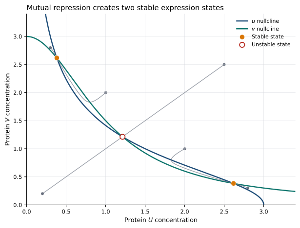
Nullclines, equilibria, and deterministic trajectories of a mutually repressing genetic toggle. — **Figure 1.** The ODE has two stable expression states, \(U\)-high and \(V\)-high, separated by the stable manifold of a saddle. In the deterministic model, each basin is permanent.

Mutual repression creates effective positive feedback: more (U) suppresses (V), and less (V) releases further production of (U). Cooperative Hill exponents make the switch sufficiently sharp for two stable asymmetric states.

This phase portrait explains the possibility of memory. It does not tell us its stochastic lifetime.

From concentrations to reaction events

Introduce a system-size parameter (\Omega) and molecular counts

U=\Omega u,\qquad V=\Omega v.

The stochastic model has four channels:

\varnothing\rightarrow U,\quad U\rightarrow\varnothing,\quad \varnothing\rightarrow V,\quad V\rightarrow\varnothing.

Their propensities are

a_1=\Omega\frac{\alpha_u}{1+(V/\Omega)^{n_v}}, \qquad a_2=\delta_u U,

a_3=\Omega\frac{\alpha_v}{1+(U/\Omega)^{n_u}}, \qquad a_4=\delta_v V.

At each Gillespie step, the total propensity determines an exponentially distributed waiting time; the relative propensities determine which event occurs. Counts remain integer and nonnegative.

Increasing (\Omega) raises copy numbers while preserving the corresponding concentration-scale drift. Relative fluctuations decrease roughly as (\Omega^{-1/2}). The deterministic ODE is therefore a large-system approximation, but no finite (\Omega) eliminates the possibility of a rare basin crossing.

Define an order parameter

m(t)=\frac{U(t)-V(t)}{U(t)+V(t)}.

Values near (+1) indicate the (U)-high state; values near (-1) indicate the (V)-high state.

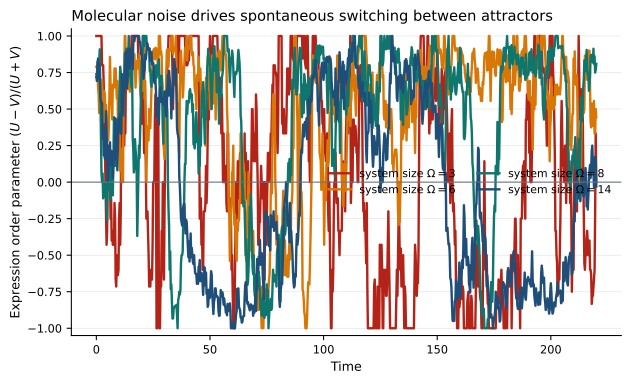
Representative stochastic toggle trajectories at molecular system sizes 3, 6, 8, and 14. — **Figure 2.** Small systems cross between expression states frequently. Larger systems spend longer near one deterministic attractor, even though the ODE phase portrait has not changed.

The state classifier uses a finite threshold beyond the separatrix. This prevents rapid recrossings near (m=0) from being counted as many independent switches.

Memory is a first-passage problem

Start every trajectory near the (U)-high equilibrium and record the first time it reaches the (V)-high region. The first-passage distribution captures both whether switching occurs within the observation window and how long it takes.

The default experiment uses 20 independent trajectories for each

\Omega\in\{3,5,8,12,18\}

over 240 dimensionless time units.

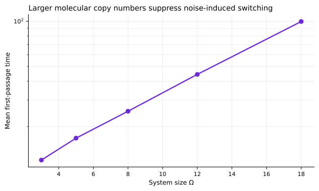
Mean first-passage time and probability of a switch within the observation window across five molecular system sizes. — **Figure 3.** Mean observed first-passage time rises with \(\Omega\). At \(\Omega=3\), every run switched and the mean was \(11.99\); at \(\Omega=18\), the mean was \(99.64\) and 85% switched within the window.

(\Omega)	Mean first-passage time	Switched within 240
3	11.99	1.00
5	16.77	1.00
8	25.30	1.00
12	44.41	1.00
18	99.64	0.85

The final row is right-censored: three of twenty trajectories had not switched by time 240. A simple mean of observed events is therefore not a complete lifetime estimator. A follow-up should use survival curves, confidence intervals, and longer horizons or rare-event methods.

The robust result is the trend, not a precise scaling law. Increasing molecular system size lengthens memory even though the deterministic equilibria are unchanged.

A stochastic equilibrium is a distribution

An ODE equilibrium is a point. A stationary stochastic state is a probability distribution over counts.

The study samples twelve long trajectories at (\Omega=8), discards an initial burn-in period, and thins the remaining samples.

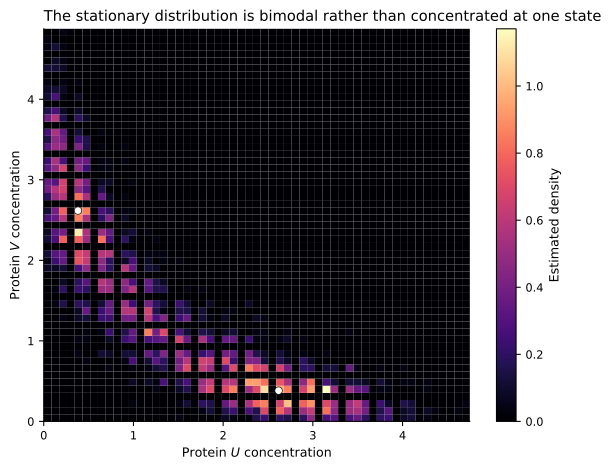
Bimodal stationary distribution of stochastic toggle states with peaks near the two deterministic equilibria. — **Figure 4.** Probability mass concentrates near the two stable ODE states. The central saddle shapes transition paths but does not become a third persistent phenotype.

This distinction prevents a common category error. “Steady state” in a stochastic model does not mean that a trajectory stops moving. It means that the distribution of possible states becomes time-invariant while individual paths continue to fluctuate and occasionally switch.

The valley between peaks contains transition states. Its probability depth is related to switching rarity, but this finite sample does not identify a quasipotential or Kramers rate.

Switching with a finite pulse

The control experiment starts in the (V)-high state and temporarily adds induction (A) to (U) production:

a_1^{\mathrm{pulse}} =\Omega\left[ \frac{\alpha_u}{1+(V/\Omega)^{n_v}}+A \right].

At (\Omega=12), pulse amplitude and duration are varied over a (5\times5) grid. Each cell uses eight stochastic replicates. The system then receives time to relax before its final state is classified.

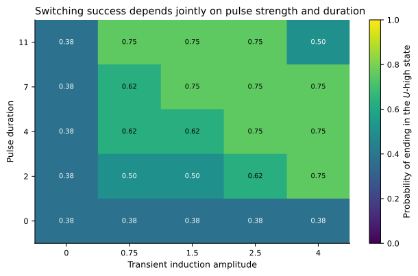
Heat map of genetic-toggle switching success over pulse amplitudes and durations. — **Figure 5.** Pulse amplitude and duration jointly determine switching probability. The best observed cell reached \(0.75\), but eight replicates per cell are too few to infer a smooth optimum.

The pulse must push the stochastic state far enough into the opposite basin that ordinary fluctuations do not immediately return it. Amplitude alone is not sufficient if exposure is too short; duration alone is weak if induction barely changes the drift.

At finite copy number, control should be formulated probabilistically:

\Pr(\text{desired state at evaluation time}\mid A,d,\Omega).

A practical design would include energy, toxicity, timing uncertainty, and a required confidence level. Bayesian binomial intervals or sequential simulation would quantify uncertainty in the success surface.

What was verified

The pipeline combines grid-based root finding, Jacobian stability classification, deterministic ODE integration, exact-event stochastic simulation, first-passage experiments, stationary sampling, and pulse-control Monte Carlo.

Three automated tests passed. They verify the number and stability of deterministic equilibria, conservation of nonnegative integer molecule counts, and reproducibility of fixed-seed stochastic paths. The output manifest contains 24 checksum-validated files.

The quoted values—three equilibria, two stable, switching probability (1.0) at the smallest (\Omega), and mean first-passage time (99.6431) at the largest—come from the validated default run.

These checks establish internal consistency, not biological validation. The Hill propensities are phenomenological; they do not explicitly model promoter binding states, transcription, or translation.

What the abstraction omits

The model assumes instantaneous regulation, equal degradation rates, and no explicit mRNA. It omits:

promoter-state switching and transcriptional bursting;
delays between transcription, translation, and repression;
cell growth, division, dilution, and molecule partitioning;
extrinsic fluctuations shared by both genes;
asymmetric production and degradation;
resource competition and growth feedback;
mutation or evolutionary stability of the circuit.

Each omission can change switching statistics. Cell division, for example, periodically halves and randomly partitions molecules; transcriptional bursting creates non-Poisson noise; delay can create oscillations or alter basin geometry.

A research path beyond brute-force Monte Carlo

The next study should separate three scales:

compute a quasipotential or minimum-action path between attractors;
use importance sampling or weighted-ensemble methods for rare switches at large (\Omega);
validate predicted lifetime scaling against direct simulation where direct simulation remains feasible.

For control, replace the coarse grid with adaptive design: choose the next amplitude–duration pair where the switching probability is most uncertain or near a target reliability. Extend the state model to include promoter switching and division, then ask whether the same pulse remains robust across cell-cycle phase.

The central conclusion is compact: bistability creates the architecture of memory; finite-copy-number noise determines its lifetime. The deterministic and stochastic models answer different questions, and using only one of them hides either the geometry or the reliability.

References

Gardner, T. S., Cantor, C. R., & Collins, J. J. (2000). Construction of a genetic toggle switch in Escherichia coli. Nature, 403, 339–342. https://doi.org/10.1038/35002131
Gillespie, D. T. (1977). Exact stochastic simulation of coupled chemical reactions. The Journal of Physical Chemistry, 81, 2340–2361. https://doi.org/10.1021/j100540a008
Segel, L. A., & Edelstein-Keshet, L. (2013). A Primer on Mathematical Models in Biology. SIAM.
McAdams, H. H., & Arkin, A. (1997). Stochastic mechanisms in gene expression. Proceedings of the National Academy of Sciences, 94, 814–819. https://doi.org/10.1073/pnas.94.3.814