Tracking Mains Noise without Losing the Muscle Signal

Surface electromyography (sEMG) is a difficult signal to condition because the thing we want and the interference we want to remove occupy overlapping worlds.

The useful waveform is stochastic, nonstationary, and spread across frequency. Power-line interference (PLI) is narrowband but not perfectly stationary: nominal 50 Hz mains can drift, develop harmonics, and couple differently across electrodes. A deep fixed notch may suppress interference, but it also removes physiological content near the notch. A heavy spectral estimator may track drift, but running it for every sample defeats a low-latency design.

This study asks a deliberately engineering-shaped question:

Can frequency-drifting harmonic interference be followed by a slow supervisory process while the sample-by-sample sEMG path remains causal, simple, and measurable?

The result is a reproducible implementation experiment, not a medical-device study. All shipped performance numbers come from controlled synthetic signals. No participant, clinical, prosthetic-control, battery, or microcontroller claim is made.

Architecture before algorithm

The pipeline runs at (f_s=2000) Hz and separates two workloads.

The fast path processes each incoming sample:

an eighth-order Butterworth band-pass represented as four second-order sections;
optional fixed notch or harmonic normalized LMS cancellation;
exponential RMS envelope estimation.

The supervisory path maintains a rolling buffer, computes an 8192-point FFT periodically, estimates the mains peak, and accepts an update only when confidence and maximum-step rules are satisfied. Its output changes oscillator frequency; it does not replace the per-sample path with a Fourier transform.

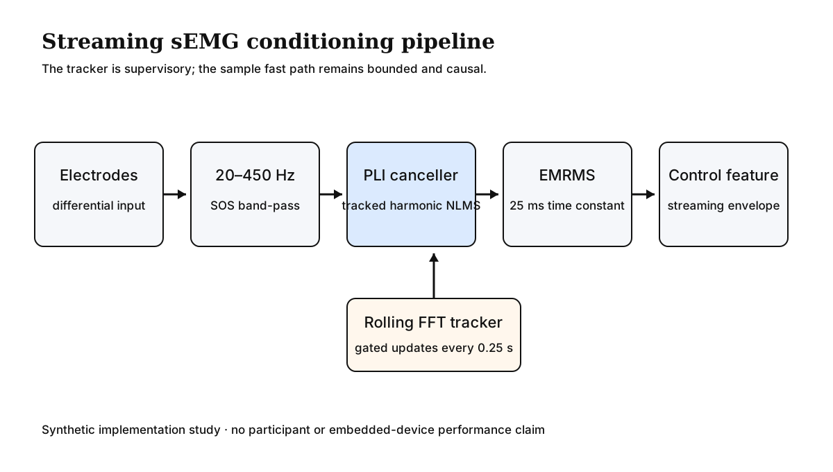
Figure 1. Separating the supervisory tracker from the causal fast path is the central architectural choice. “Low latency” is measured for the fast path; accepted tracker updates are timed and reported separately.

This separation prevents a common reporting error. Averaging an occasional expensive FFT over thousands of cheap samples may produce a small mean time while hiding a large supervisory spike. Conversely, quoting the FFT time as though it occurred for every sample understates throughput. The implementation records fast-path time, total synchronous host time, and accepted tracker-update time as different quantities.

From common-mode voltage to differential interference

Electrodes are intended to reject voltage shared by both inputs, but finite common-mode rejection converts some of it into a differential contaminant. If the two input gains are (G_1) and (G_2), a simplified decomposition gives

v_{\mathrm{out}} = G_d\,v_d+G_c\,v_c, \qquad \mathrm{CMRR} =20\log_{10}\left|\frac{G_d}{G_c}\right|.

A large CMRR helps, but it is not a complete PLI model. Electrode impedance imbalance, cable motion, capacitive coupling, reference placement, and frequency-dependent front-end behaviour all matter. The project’s CMRR screen is therefore a sensitivity analysis: it explains why a nominally common-mode sinusoid may remain after differential acquisition, without pretending to identify a particular hardware path.

Digital cancellation comes after this analogue limitation. It cannot restore information that saturated the amplifier, and it should not be treated as permission to ignore electrode preparation or front-end design.

Why a static notch is an incomplete answer

A second-order notch centred at angular frequency (\omega_0) can place zeros on the unit circle:

H(z) = \frac{1-2\cos(\omega_0)z^{-1}+z^{-2}} {1-2r\cos(\omega_0)z^{-1}+r^2z^{-2}},

where (r<1) controls the pole radius and bandwidth. A narrow notch preserves more neighbouring spectrum but becomes sensitive to frequency drift. A wide notch tolerates drift at the price of suppressing more sEMG content and adding phase distortion.

Harmonics complicate the trade-off. Interference at 100 Hz can remain even if the fundamental is well suppressed. Cascading several wide notches creates a comb of removed physiological bands. The alternative tested here is to synthesise reference sinusoids at the tracked fundamental and its harmonics, then adapt their amplitudes.

Harmonic normalized LMS

For harmonic (k), the reference pair is

\mathbf x_{k,n} = \begin{bmatrix} \sin(k\phi_n)\\ \cos(k\phi_n) \end{bmatrix}, \qquad \phi_{n+1} = \phi_n+\frac{2\pi\widehat f_n}{f_s}.

Recursive quadrature oscillators update these references without evaluating sine and cosine for every sample. Concatenating the pairs gives (\mathbf x_n); the estimated interference is

\widehat i_n=\mathbf w_n^\top\mathbf x_n, \qquad e_n=y_n-\widehat i_n.

The normalized LMS update is

\mathbf w_{n+1} = \mathbf w_n +\mu\, \frac{e_n\mathbf x_n} {\varepsilon+\lVert\mathbf x_n\rVert^2}.

Normalisation makes the step less sensitive to reference magnitude, but (\mu) still controls a real trade-off. A small value follows amplitude changes slowly; a large value converges quickly but can begin fitting signal components correlated with the reference. The supplied sensitivity experiment compares (\mu\in{0.005,0.02,0.08}) rather than declaring one universal optimum.

The frequency tracker is allowed to say “not sure”

The supervisory tracker searches around nominal mains frequency and uses spectral concentration to score confidence. A candidate update is accepted only if:

confidence exceeds 2.5;
smoothing with factor 0.5 is applied;
the accepted change is at most 0.25 Hz per supervisory step.

Low-confidence estimates leave the oscillator at its previous frequency. This is important. A tracker forced to emit a new value from every noisy window can inject frequency jitter into the canceller and make it chase broadband sEMG.

The 8192-point FFT does not imply raw-bin resolution is the final estimate. Peak interpolation can give sub-bin estimates, while window length still controls the amount of history and the ability to follow rapid drift. In the synthetic tracking run, the true interference spans approximately (49.859) to (50.516) Hz and tracker RMSE is (0.118) Hz.

What the synthetic ablation shows

Two declared synthetic benchmarks answer different questions.

The 12-channel ablation compares cancellation modes against a known clean reference. Median reconstruction SNR is:

Mode	Median reconstruction SNR
Cancellation off	(-11.19) dB
Fixed harmonic	(8.80) dB
Tracked harmonic	(11.48) dB

Envelope alignment after the declared lag convention gives correlation (0.9943) and normalized RMSE (0.0693).

The drifting-mains experiment focuses on tracking. During activity intervals, reconstruction SNR is (-15.68) dB for a static notch, (-2.33) dB for fixed harmonic cancellation, and (3.53) dB for tracked harmonic cancellation. The median rest envelope is (492.7), (88.6), and (74.6\ \mu\mathrm V), respectively.

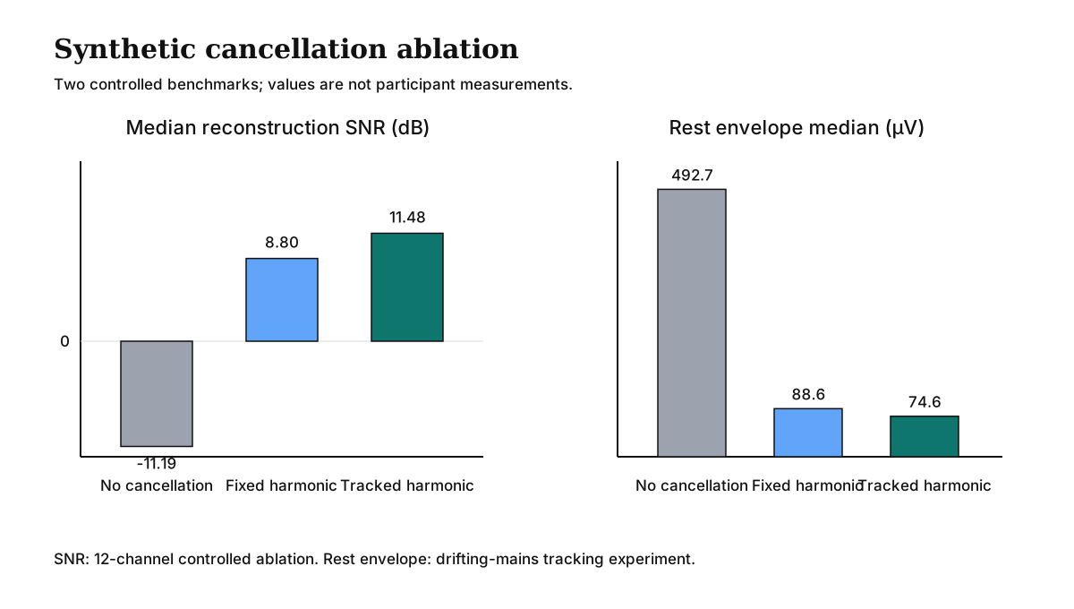
Bar charts comparing synthetic reconstruction SNR and residual rest-envelope amplitude for cancellation off, fixed harmonic, and tracked harmonic modes. — **Figure 2.** Tracked harmonic cancellation performs best in the two supplied synthetic benchmarks. The panels use different experiments and metrics; neither is participant evidence.

The gains should not be compressed into “the algorithm improves sEMG by 11.5 dB.” That value is conditional on the synthetic interference, clean reference, amplitude distribution, startup exclusion, and reconstruction metric. Real recordings do not provide a perfectly known clean counterfactual.

Envelope estimation is a latency choice

The exponential mean-square state is

q_n=(1-\alpha)q_{n-1}+\alpha e_n^2, \qquad \mathrm{EMRMS}_n=\sqrt{q_n},

with

\alpha=1-\exp\left(-\frac{1}{f_s\tau}\right).

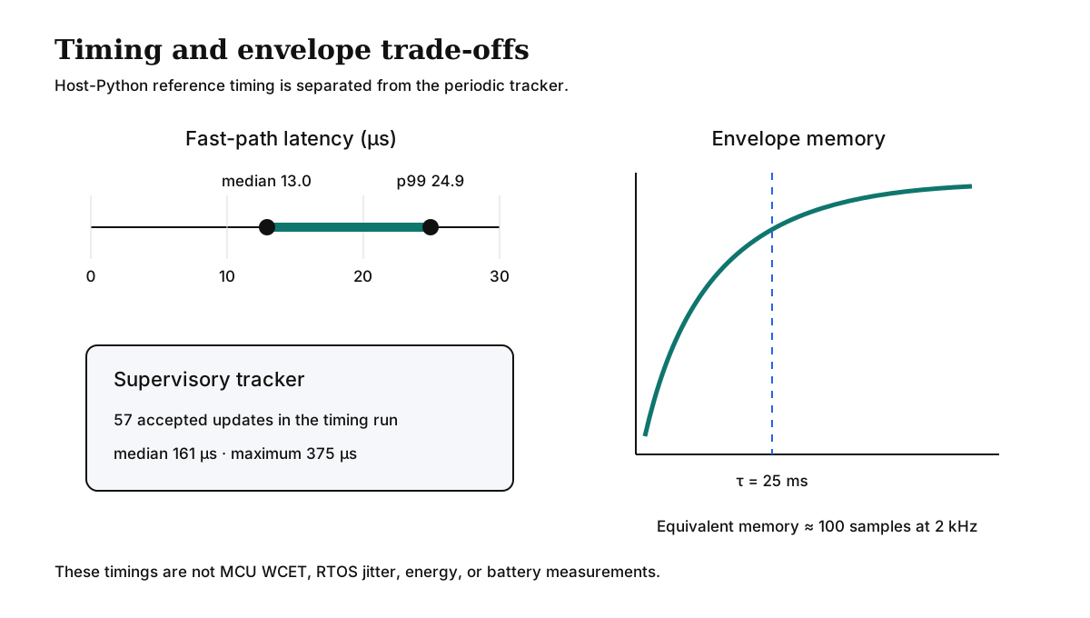
At (f_s=2000) Hz and (\tau=25) ms, the equivalent memory is roughly 100 samples. A smaller (\tau) responds faster but produces a noisier control feature; a larger (\tau) stabilises amplitude while delaying onset and offset.

Startup correction also needs explicit indexing. With zero-based sample index (n), the accumulated weight is (1-(1-\alpha)^{n+1}). Using (n) instead of (n+1) creates an avoidable transient error.

The study compares EMRMS with a rectangular running RMS implemented by a rolling sum. Both can have constant arithmetic cost per sample; the distinction is their temporal weighting, memory, and delay—not a simplistic claim that one is “real time” and the other is not.

Timing: what was measured

The reference benchmark processes 30,000 samples on host Python. Reported times are:

Workload	Median	99th percentile
Sample fast path	(12.96\ \mu s)	(24.94\ \mu s)
Total synchronous call	(13.64\ \mu s)	(26.56\ \mu s)
Accepted tracker update	(161.15\ \mu s)	reported separately

There were 57 accepted tracker updates in that run; the maximum tracker time was (375.45\ \mu s). These are reference measurements from Python 3.13.5 on one Linux host. They are not worst-case execution time, RTOS jitter, interrupt latency, memory bandwidth, power, thermal, or battery measurements.

Host-Python sample-fast-path timing interval and a diagram of the 25 millisecond exponential RMS memory. — **Figure 3.** Timing and smoothing answer different design questions. The fast path fits comfortably inside a 500-microsecond sample period in this host reference, but only an embedded implementation can establish device-level deadlines.

The Ninapro boundary

The private source workspace includes a real-data validation command that requires legitimate local Ninapro DB2 MAT files and exits when none are found. The shipped performance summaries are explicitly synthetic.

One legacy output is named ninapro_summary.json, but its own data_source says “Ninapro-like synthetic stand-in.” This article does not treat it as Ninapro validation and does not quote its results as participant evidence. File names are not provenance.

A valid real-data study would need documented dataset version and license, subject-level separation, verified unit scaling, channel and exercise selection, artefact policy, and a metric that does not require an unavailable clean signal. Cross-validation must split by subject or session when the intended claim is generalisation, not randomly mix neighbouring windows.

What ten tests do—and do not—establish

Ten tests passed in the source implementation. They cover filter behaviour, exponential RMS definitions, correction indexing, and pipeline operation. Deterministic figure generation and machine-readable JSON reduce transcription errors.

Tests establish consistency with the declared numerical design. They do not establish clinical usefulness, hardware safety, electromagnetic compatibility, or robustness to sweat, electrode lift, movement artefact, saturation, and adversarial signal overlap.

A concrete route to stronger evidence

The next study should freeze the current synthetic pipeline before looking at real outcomes, then proceed in layers:

acquire or lawfully access a named dataset and verify physical units;
define subject-level train, tuning, and held-out splits;
compare static notch, fixed harmonic, tracked harmonic, and no-cancellation baselines;
report signal-quality proxies that remain meaningful without a clean reference;
implement the frozen fast path on a target MCU and measure WCET, jitter, memory, energy, and numerical precision;
test failure gates for low confidence, missing windows, clipping, and rapid interference shifts;
only then evaluate task-level consequences such as gesture classification or proportional control.

That programme would convert a reproducible mechanism study into evidence about a real acquisition and deployment context. Until then, the honest result is narrower and still useful: a tracked supervisory oscillator can improve controlled harmonic cancellation without placing spectral estimation in every sample step.

References

Widrow, B., Glover, J. R., McCool, J. M., et al. (1975). Adaptive noise cancelling: Principles and applications. Proceedings of the IEEE, 63(12), 1692–1716. https://doi.org/10.1109/PROC.1975.10036
De Luca, C. J., Donald Gilmore, L., Kuznetsov, M., & Roy, S. H. (2010). Filtering the surface EMG signal: Movement artifact and baseline noise contamination. Journal of Biomechanics, 43(8), 1573–1579. https://doi.org/10.1016/j.jbiomech.2010.01.027
Clancy, E. A., Morin, E. L., & Merletti, R. (2002). Sampling, noise-reduction and amplitude estimation issues in surface electromyography. Journal of Electromyography and Kinesiology, 12(1), 1–16. https://doi.org/10.1016/S1050-6411(01)00033-5
Merletti, R., & Farina, D. (Eds.). (2016). Surface Electromyography: Physiology, Engineering, and Applications. Wiley. https://doi.org/10.1002/9781119082934
Atzori, M., Gijsberts, A., Castellini, C., et al. (2014). Electromyography data for non-invasive naturally-controlled robotic hand prostheses. Scientific Data, 1, 140053. https://doi.org/10.1038/sdata.2014.53