When Local Precision Hides the Wrong Heat Source

Imagine placing a thermometer halfway along an insulated rod. A short heat pulse occurs somewhere inside it, and you record the temperature as the disturbance spreads. The curve is smooth. A fitted model reproduces it closely. The derivatives of that model are independent, and the local uncertainty calculation looks reassuring. Have you found the source?

Not necessarily. A pulse on the left and its reflection on the right can produce exactly the same midpoint record. This is not a shortage of decimal places, an unfortunate random sample or a solver that needs a few more iterations. Under the symmetric experiment, the distinguishing information never reaches the output in the first place. A locally narrow explanation can sit beside a distant, equally valid explanation.

This is a hypothetical sensing problem, not a fire experiment or an engineering deployment. The model below deliberately makes the physics simple enough to check: one initial pulse, one spatial dimension, reflecting boundaries and an explicit heat kernel. That simplicity lets us ask a harder design question without hiding it behind a large numerical simulator. If there are only eight readings to spend, should we concentrate on local precision, spread measurements evenly, break a particular symmetry, or protect against distant competing sources?

The answer from this finite study is conditional. The midpoint counterexample is exact, but it does not mean that ordinary design methods fail whenever a problem is nonlinear. At zero delay, all six tested two-sensor layouts avoided the declared large location error; equal spacing even had a smaller median error than the maximin layout. Delayed measurements were more difficult, and the more elaborate objectives did not remove that difficulty. The useful lesson is to choose an experiment for the question it must answer—not to replace one universal score with another.

What does the thermometer actually observe?

The rod is represented by the dimensionless interval $0<x<1$ . Temperature evolves according to a heat equation with diffusion coefficient $D>0$ . The boundaries reflect heat rather than letting it escape, and the pulse time is known. If the pulse has positive strength $A$ and location $a$ , the mathematical model is

u_t=D u_{xx},\qquad u_x(0,t)=u_x(1,t)=0,\qquad u(x,0)=A\delta(x-a).

The delta symbol describes an ideal localized initial input. It does not mean that an ordinary thermometer measures an infinite temperature at time zero: every observation here has strictly positive time. Nor is this an always-on heater. A continuously acting source would enter the differential equation as forcing and produce a different forward map. This distinction matters when comparing studies of heat-source reconstruction [6,8,9].

An insulated interval has cosine eigenfunctions. Expanding the solution in those modes gives

u(x,t;A,a,D)=A K_D(x,t;a),\qquad K_D(x,t;a)=1+2\sum_{n=1}^{\infty}\cos(n\pi x)\cos(n\pi a)e^{-Dn^2\pi^2t}.

Each mode contains three pieces: where the sensor sits, where the pulse occurred and how much diffusion has damped that spatial pattern by the observation time. The constant term preserves the total heat. Integrating over the rod makes all nonconstant cosine modes vanish, so the integral of $u$ remains $A$ . A later temperature close to $A$ is therefore compatible with substantial loss of source-location information: conservation of heat is not conservation of every spatial detail.

For eight specified sensor-time pairs, collect the predicted readings into a vector $\mu_\xi(A,a,D)$ , where $\xi$ denotes the experimental layout. Observed values are

y_i=A K_D(x_i,t_i;a)+\varepsilon_i,\qquad \varepsilon_i\ \mathop{\sim}^{\mathrm{iid}}\ N(0,\sigma^2).

The fixed Gaussian standard deviation is a study assumption, not a calibrated sensor specification. The positions are known, the channels retain their labels, and the pulse onset is known. These choices keep the benchmark interpretable, but they also define what its conclusions cannot cover.

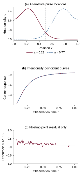
Mirror heat fields differ away from the center, but center time series coincide; a separate panel shows floating-point roundoff. — Figure 1. Two alternative initial pulses, not two simultaneous sources. With A=1 and D=0.05 on the reflecting unit interval, the t=0.24 heat fields differ while their x=0.5 time series coincide analytically. The final panel exposes only finite-precision evaluation residuals; the curves in the middle panel overlap intentionally. All quantities are dimensionless.

The information that reflection removes

At the midpoint, $\cos(n\pi/2)=0$ for every odd $n$ . For even modes, reflecting the source from $a$ to $1-a$ leaves its cosine coefficient unchanged. Consequently,

K_D(1/2,t;a)=K_D(1/2,t;1-a),\qquad t>0.

This identity holds for every positive time and every positive $D$ . It also survives unknown amplitude: the two reflected explanations can use the same $A$ . Even an arbitrarily long, noiseless midpoint time series cannot choose between them. Repeating a blind measurement more accurately may shrink numerical fluctuations, but it does not remove a structural symmetry of the observation map.

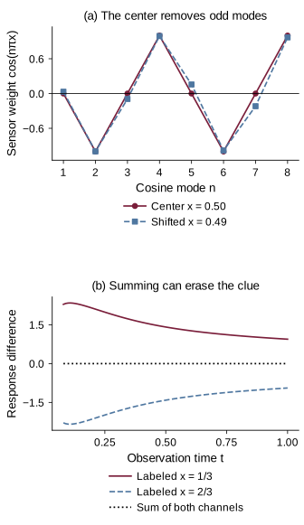
Away from the midpoint, the reflected difference contains only the odd modes:

K_D(x,t;a)-K_D(x,t;1-a) =4\sum_{\substack{n\ge1\\n\ \mathrm{odd}}}\cos(n\pi x)\cos(n\pi a)e^{-Dn^2\pi^2t}.

This formula says exactly what moving the sensor can recover. It does not say that every off-center sensor identifies every continuous source stably under noise. A surviving difference can still be small, and another choice of amplitude or diffusivity may mimic part of it. Breaking one exact symmetry is the beginning of a design analysis, not the end.

There is a second, easily missed distinction. Two labeled sensors at reflected positions need not be blind. A reflected source exchanges their output blocks; it does not usually preserve the ordered observation vector. In a numerical control, the labeled response distance is about 4.50148, whereas summing the paired channels restores equality to rounding precision. A physically symmetric layout can be informative because the instrument tells us which side produced each reading. Discarding that label changes the experiment.

Cosine weights show odd-mode removal; labeled symmetric channels distinguish mirrors but their sum does not. — Figure 2. Odd cosine modes have exactly zero midpoint weight; moving to x=0.49 retains some of them. For the two alternative sources 0.23 and 0.77 with A=1,D=0.05, the labeled measurements at 1/3 and 2/3 are different: reflection swaps the channels. Their sum removes this distinguishing contrast. Thus a spatially symmetric pair of labeled sensors is not inherently aliased; aggregation is a different observation operator.

Why a full-rank Jacobian does not settle the question

Local information asks what changes when parameters move a little around one nominated explanation. For known $D$ and parameters $(A,a)$ , the Jacobian columns are $K_D$ and $A\partial_aK_D$ . With independent Gaussian measurement errors, the Fisher information matrix is

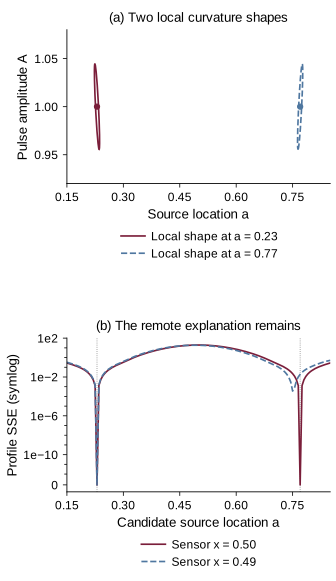
J_i=\left[K_D(x_i,t_i;a),\ A\partial_a K_D(x_i,t_i;a)\right],\qquad F=\frac{J^{\mathsf T}J}{\sigma^2}.

At the frozen midpoint example, the smallest eigenvalue is approximately 498.237, not zero. The local effects of changing the pulse strength and nudging the source position are independent across the selected times. Yet the source at 0.77 remains an exact alternative to the source at 0.23. The two statements are consistent because a move of 0.54 is not an infinitesimal perturbation around the original explanation.

One can picture the set of possible observation vectors as a surface in measurement space. A full-rank derivative means that the surface has the expected local tangent directions at a point. It does not prevent another, distant part of the parameter domain from arriving at the same observation. Pázman and Pronzato studied precisely this broader design problem: locally informative nonlinear models can fold back toward distant explanations, motivating criteria based on response secants rather than tangents alone [1].

Allowing $D$ to be unknown does not repair the midpoint symmetry. The extended Jacobian has a third column, $A\partial_DK_D$ . At the same frozen case its computed information eigenvalues are approximately 119.854, 3,874.053 and 235,504.067, all positive, while the exact reflected identity remains. These are local values under that coordinate convention, not scores to compare numerically with the earlier two-parameter eigenvalues.

Fisher information is not being disproved. It answers a local question very well. The mistake would be to read its curvature ellipse as a complete, globally valid confidence region without checking whether the data admit other branches. A single ellipse cannot display a disconnected alternative that the approximation never considered.

Figure 3. At a midpoint sensor, both separated source locations have nonsingular local Fisher information for unknown (A,a) with D=0.05 and eight fixed times. The upper contours show unit local information geometry, not calibrated global confidence regions. The lower plot profiles A in [0.7,1.3] for noiseless data from a=0.23. Midpoint sampling retains both minima; displacement to 0.49 removes this particular mirror fit. Symlog displays zero without adding an artificial positive residual.

An oracle that knows exactly two explanations

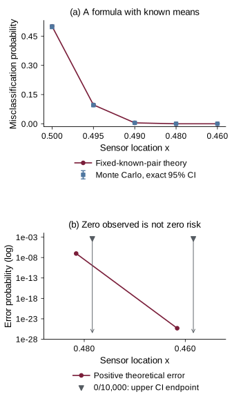
Before introducing nuisance parameters, there is a useful statistical control. Suppose the only possibilities are two fixed, specified mean vectors $\mu_0$ and $\mu_1$ , both with covariance $\sigma^2 I$ and equal prior probability. The best classifier compares the two Gaussian likelihoods. Its exact error probability is

P_{\mathrm{err}}^*=\Phi\!\left(-\frac{\|\mu_1-\mu_0\|_2}{2\sigma}\right).

Here $\Phi$ is the standard normal cumulative distribution function. Coincident means give error one half. Widely separated means give small error. The distance is measured relative to noise across the entire observation vector, not just the largest separation at one time.

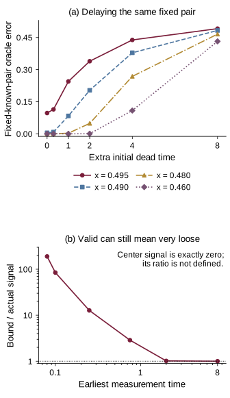
With $A=1$ , $D=0.05$ , $\sigma=0.05$ and the original eight times, moving the sensor from 0.5 to 0.495 changes the fixed-pair theoretical error from 0.5 to about 0.096995. At 0.49 it is about 0.004677. The corresponding seeded counts are 4,979, 956 and 47 errors out of 10,000. These calculations verify the implementation against an independently known probability law. They do not create evidence that the Gaussian law or heat-source inversion is new.

At sensors 0.48 and 0.46, the simulation records zero errors out of 10,000, but the theoretical probabilities remain positive. A zero count is not zero risk. The two-sided 95% Clopper–Pearson interval has an upper endpoint about 0.00036882 in each zero-count case, rather than collapsing to zero. This is an ordinary finite-sample interval for repeated classification trials under the fixed sensor, hypothesis pair and noise model, with equal-prior class labels.

The oracle has been granted knowledge that a real inverse analysis may not possess: both amplitudes, both diffusivities and the two possible locations. Once those quantities become unknown, the formula no longer gives the error of the resulting composite classifier. It is a deliberately simpler reference, not an answer to every later question.

Known-pair oracle probabilities agree with Monte Carlo; zero-error trials retain positive confidence upper endpoints. — Figure 4. The exact Gaussian formula applies only to equal-prior hypotheses with both means fully specified: A=1,D=0.05,a=0.23 or 0.77, eight readings, sigma=0.05. Each sensor has 10,000 seeded trials; error bars are pointwise two-sided Clopper–Pearson intervals. For zero observed errors, downward triangles mark only the positive upper interval endpoint, not an estimated probability at that height. Arrows indicate continuation toward zero; their graphical tips are not positive lower confidence bounds. These are not error guarantees for unknown-amplitude/diffusivity inversion.

Unknown strength is more than a wider error bar

A different source position need not imitate the true signal using the same strength. For a candidate location and diffusivity, write $k$ for its unit-amplitude response vector. The best strength within the declared bounds has a simple expression:

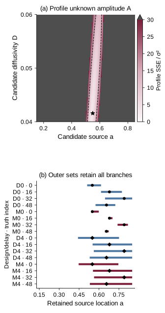
\widehat A(a,D)=\operatorname{clip}_{[0.7,1.3]} \left(\frac{k(a,D)^{\mathsf T}y}{k(a,D)^{\mathsf T}k(a,D)}\right).

Substituting it into the residual gives a profile surface over $(a,D)$ . This removes a linear nuisance variable exactly; it does not make the remaining problem convex. Multiple basins may survive. A noiseless midpoint profile has equal reflected minima even after amplitude has been optimized. Off-center data can change that landscape, but a low residual at one candidate does not tell us what the rest of the landscape contains.

Diffusivity introduces a different compensation. The factors $e^{-Dn^2\pi^2t}$ determine how quickly spatial details decay. A distant candidate can alter both the amount of heat and the speed with which its pattern smooths. In a genuine ambiguity audit, that alternative must be allowed its own $A'$ and $D'$ . Requiring the competing explanation to use the true nuisance values would silently make the task easier.

The study therefore restricts $A$ to $[0.7,1.3]$ , $a$ to $[0.15,0.85]$ and $D$ to $[0.04,0.06]$ . These are explicit prior bounds, not values learned from field data. A positive amplitude floor matters: if arbitrarily weak sources were permitted, all layouts could face nearly zero signals. Likewise, any continuous source domain contains arbitrarily close pairs, so a nonzero minimum distance cannot be demanded without specifying how far apart the competing locations must be.

The numerical inverse solver profiles amplitude on an 81-by-41 location/diffusivity grid, retains multiple basins and a reflected candidate, then applies bounded continuous refinement. Every final residual is recomputed directly. This is a stronger diagnostic than reporting one optimizer run, but it still is not a proof of global minimization. A successful stopping message, a low residual and a globally exhaustive search are different achievements.

Unknown-amplitude point-source recovery already has a substantial literature. Huynh and colleagues, for example, analyze sensor-dependent reconstruction error for sources represented as measures under explicit noise and nondegeneracy assumptions [7]. The present three-parameter model does not replace that theory. Its role is to make the compensation between a few physical parameters visible, with enough independent controls to tell an observation problem from a numerical one.

Figure 5. The upper surface uses the predeclared first held-out truth, noise replicate zero, local-D design and zero delay; A is profiled in [0.7,1.3]. The dashed contour is the eight-dimensional noise-ball cutoff, not a one-degree-of-freedom likelihood-ratio contour. Values above 30 use the overflow color. D/M denote local-D/maximin; labels give delay and truth index. Solid bars are retained intervals; black circles/diamonds mark generating locations at delay 0/4. Here 16/16 outer projections are connected and 16/16 retain the generating location; 0 hit the resource cap. Width-stop unresolved boxes are retained. Model-based 95% coverage is pointwise, not simultaneous.

Eight readings, six ways of spending them

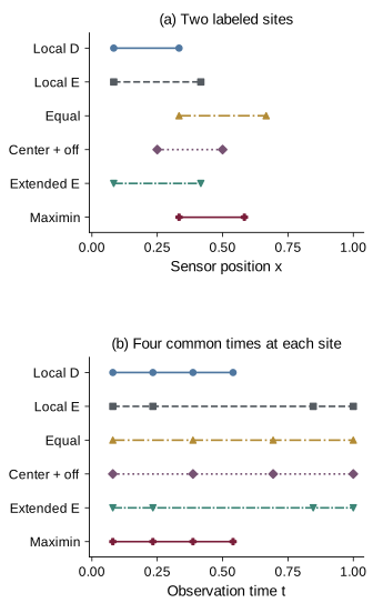
The main design comparison has a fixed hardware and measurement budget: two distinct labeled sensors, each observed at four common times. Eleven possible positions are $j/12$ for $j=1,\ldots,11$ . Seven possible times are $\tau+0.08+0.92j/6$ , where $j=0,\ldots,6$ . Choosing two positions and four times gives exactly 1,925 feasible layouts for each dead time. They can all be enumerated rather than relying on a lucky layout optimizer.

Dead time $\tau$ is the initial interval during which no readings are available. It is not a sensor recovery interval between samples. The main cases use $\tau=0,1,4$ , always with the same duration of accessible observation window after startup. The original single midpoint sensor with eight readings remains a structural control, but it is not ranked as if it used the same two-sensor hardware.

Local D-opt maximizes the log determinant of the three-parameter information matrix at the frozen nominal point $(1,0.23,0.05)$ . Local E-opt maximizes its smallest eigenvalue. Neither is allowed to recenter at each held-out truth. Fixed parameter scales of 0.3, 0.35 and 0.01 make the coordinate convention explicit; especially for E-opt, changing units without declaring them can change which direction appears weakest.

An equal-spacing baseline uses sensors at $1/3$ and $2/3$ , with four equally spaced times. A pre-fixed center-plus-off-center control uses $1/4$ and $1/2$ at the same times. The latter tests a straightforward engineering idea—retain a common central reference while adding an asymmetric observation. It is not advertised as the best possible symmetry-aware design.

The fifth method is a discretized extended-E criterion based on existing globalized design theory [1]. It compares responses to a nominal anchor while dividing by squared scaled parameter distance. The anchor and denominator matter: an unnormalized pair-distance objective is not the same criterion. Its finite parameter grid is a declared approximation, not a complete reimplementation of a published continuous optimization method.

The sixth method maximizes the smallest profiled response separation between well-separated source explanations on the design grid. Robust model discrimination has long considered unknown competing-model parameters [2,3], and strict-budget robust PDE design has substantial prior theory [5]. This experiment uses those ideas to ask a model-specific comparison, not to announce a new optimal-design principle.

The word global also needs care. Qi and Baker compare Fisher information with Sobol-based global sensitivity in noisy observation-time design [4]. Sensitivity integrated over a parameter distribution is not the same thing as proving that no distant parameter pair overlaps. Likewise, modern multi-type PDE sensor design can optimize information gain under heterogeneous costs [10]; this benchmark deliberately uses identical readout costs and does not borrow those frameworks’ approximation guarantees. Similar vocabulary does not make distinct objectives interchangeable.

The six selected sensor pairs and common four-time schedules all use exactly eight readings. — Figure 6. Six zero-delay layouts share two fixed labeled sensors and four common times, totaling eight readings. Local-D, local-E, discrete extended-E and maximin are selected from the same 1,925 candidates using only frozen design information; equal spacing and center-plus-off-center are pre-fixed engineering controls. Repeated layouts are retained rather than treated as independent evidence. Each site in the upper panel receives every time shown for its method below.

What does “globally separated” mean here?

Let $\Delta=0.2$ denote the location error scale of interest. A design’s task-specific separation is

\beta_\Delta(\xi)= \inf_{\substack{a,a'\in[0.15,0.85]\\|a-a'|\ge\Delta\\A,A'\in[0.7,1.3]\\D,D'\in[0.04,0.06]}} \frac{\|\mu_\xi(A,a,D)-\mu_\xi(A',a',D')\|_2}{\sigma}.

The two diffusivities describe competing explanations of one unknown experiment, not two materials simultaneously changing inside the rod. Each explanation uses one common amplitude and diffusivity across its entire reading vector, not a fresh pair for every observation. The lower amplitude bound and nonzero location separation prevent two trivial routes to a zero objective. A positive value would rule out sufficiently distant near-coincident means within this box; it would not prove injectivity at every arbitrarily small location scale.

For fixed kernel vectors $v,w$ , both nuisance amplitudes can be eliminated by a bounded quadratic calculation. At least one optimal amplitude can be chosen at its lower bound: otherwise simultaneously reducing both decreases a nonzero response difference. Checking the two lower-bound edges gives the minimum without a coarse amplitude grid. The remaining source locations and diffusivities still require a global search or enclosure.

For design selection, the source grid includes eight locations from 0.15 to 0.85 in steps of 0.1, plus 0.23 and 0.77; diffusivities are 0.04, 0.05 and 0.06. The maximin design is optimal only within the declared finite layout family and this parameter-grid criterion. It is not globally optimal over arbitrary sensor trajectories, arbitrary times or all continuous parameter uncertainty.

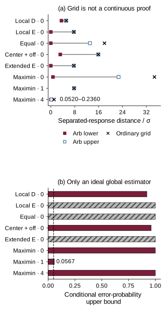
There is a particularly important inequality direction. Minimizing over a finite subset cannot find a value below the true continuous minimum unless a numerical error is involved. The grid result is therefore an upper bound on the continuous worst-case separation. A large grid value can motivate further investigation, but by itself it cannot certify that an unsampled pair is not much harder.

At zero delay the grid raw distances are about 0.257568 for local D-opt, 0.385917 for local E-opt and extended-E, 0.898403 for equal spacing, 0.795387 for the center-plus-off-center control and 1.735078 for maximin. These are noise-unscaled distances, not error probabilities. Maximin winning the score it maximizes is unsurprising; the scientific question is whether that advantage survives the change of question and the change of parameter set.

The worst pair need not be the headline mirror example. For zero-delay local D-opt, the two sites are $1/12$ and $1/3$ ; its grid witness compares $(A,a,D)=(0.7,0.65,0.04)$ with $(1.3,0.85,0.06)$ . The alternative compensates using both nuisance parameters. Maximin instead selects $1/3$ and $7/12$ and has a different worst pair. A design can solve the obvious left/right control while leaving another part of its source domain relatively weak. That is why the full domain, not just a visually persuasive example, enters the comparison.

What happened away from the design grid?

Sixty-four frozen Sobol parameter combinations supply held-out truths inside the stated box. Each has 32 independent Gaussian noise vectors, shared across methods. They are fixed benchmark cases, not 64 independent draws from a population of physical rods. At zero delay, the three noise levels are 0.025, 0.05 and 0.1; delayed experiments use 0.05. Six methods across these settings produce 30 conditions and 61,440 continuous inverse fits.

The main large-error indicator is $|\widehat a-a|\ge0.2$ . It is a declared research scale, not a universal engineering tolerance. Median error reports typical numerical location accuracy, while the large-error count asks whether the procedure chose a substantially distant answer. Both are worth seeing because a ranking can change when the target changes.

At $\tau=0$ and $\sigma=0.05$ , each method has 2,048 fits and zero large location errors. The medians are nevertheless different. Equal spacing gives about 0.00246372, the center-plus-off-center control 0.00289780, maximin 0.00311622, local E-opt and extended-E 0.00347328, and local D-opt 0.00608662. The simplest layout is best by that particular summary, despite its smaller optimized-grid separation.

This negative result matters: midpoint ambiguity does not predict failure of locally optimized, labeled two-sensor layouts. Protecting a worst pair and minimizing median error are different design targets.

At $\tau=1$ , all six layouts still record zero large location errors, although their median errors increase. At $\tau=4$ , the counts become 31 for local D-opt, local E-opt and extended-E, 72 for equal spacing, 124 for the fixed center-plus-off-center layout and 29 for maximin, each out of 2,048. The two-count difference between maximin and the local criteria is not presented as a universal or statistically established superiority claim. The data are paired and the layouts may coincide.

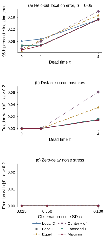
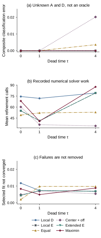
Held-out 95th-percentile location errors and distant-source mistake fractions vary across delay and noise, with all fits retained. — Figure 7. Each condition retains 64 fixed held-out parameter sites and 32 paired independent noise vectors per site (2,048 fits). The upper statistic is a finite-benchmark 95th percentile, not a confidence limit; lower fractions count distant location errors at scale 0.2. No population confidence intervals are inferred from Sobol sites. Unsuccessful numerical optimizers remain in the denominators. Some local/extended-E curves overlap intentionally because they select the same physical layout; this is not replication evidence.

The separate composite classifier receives two possible locations but not their strengths or diffusivities. It profiles both nuisances under each hypothesis. Three mirror pairs, two labels, two strengths, two diffusivities and 128 noise realizations give 3,072 decisions per condition, or 92,160 overall. At delay four, equal spacing records 11 wrong decisions and the center-plus-off-center control 62; the other four criteria record zero. All earlier composite conditions also record zero.

Choosing between two specified positions can be easier than continuous localization with compensating nuisance parameters. The classifier and inverse solver have different candidate sets and outputs; their error counts answer different questions.

Zero also has to retain its denominator. With zero errors in $n$ repetitions of one fixed-truth experiment, the two-sided 95% exact upper endpoint is

p_{\mathrm{upper}}=1-0.025^{1/n}.

For 32 noise repetitions it is about 0.108881. Pooling all 2,048 outcomes mixes 64 potentially different error probabilities; it does not establish a common zero risk at every source. The per-truth intervals and finite counts answer the modest question the experiment actually repeats, without treating time points or parameter-grid locations as interchangeable independent evidence.

A certificate must cover the space between grid points

A continuous lower bound needs something more than denser plotting. For selected final layouts, the calculation encloses the heat kernel and its derivatives with outward-rounded real-ball arithmetic, includes explicit infinite-series tails and subdivides the four nonlinear source/diffusivity coordinates. Amplitude profiling remains bounded. Every retained cell contributes a lower bound; feasible parameter witnesses contribute upper bounds.

The process has a fixed 50,000-cell work cap and a target raw distance width of $10^{-6}$ . Any unprocessed feasible region remains represented. If the lower endpoint is zero while the upper endpoint is positive, the result is unresolved at that work budget, not a proof that an exact alias exists. Conversely, a positive lower endpoint certifies only the declared separation problem, not the truth of the model itself.

Simulation checks finitely many truths; the lower bound must survive every admissible distant competitor. That costs more, and a mathematically valid bound can still be too conservative to support a useful statistical conclusion.

Suppose an independently verified raw lower distance is $b$ . For an ideal exact global nearest-model estimator, the triangle inequality gives a simple conservative implication: a sufficiently small noise vector prevents a location error of size $\Delta$ . Under the frozen Gaussian model,

\Pr\!\left(|\widehat a-a|\ge\Delta\right) \le \Pr\!\left(\chi^2_8\ge\frac{b^2}{4\sigma^2}\right).

This is not the two-fixed-mean Gaussian oracle. It is also not automatically a bound for the numerical profile solver used in the empirical comparison, because that solver has not been certified as an exact global minimizer for every noisy vector. The distinction prevents a useful mathematical implication from being attached to an algorithm that has not met its assumptions.

All eight enclosure calculations reach the work cap before the target width. Five retain positive separation lower bounds; three remain unresolved at zero. At zero delay, local D-opt gives a raw enclosure [0.178777,0.257569], while maximin gives [0.036311,1.134591], with displayed endpoints rounded outward. These overlapping enclosures have different sharpness and cannot rank the designs. For maximin at delay one, the enclosure narrows to [0.388936,0.389382], yet the sufficient ideal-estimator error bound is about 0.056719, still above a 5% target. At delay four that bound is essentially one. None of the eight establishes the 5% target. A tighter certificate can describe a worse experiment; an uninformative sufficient bound does not prove classification impossible.

A complementary uncertainty display uses the observation noise directly. With $\Theta$ denoting the declared compact parameter box, define

C(y)=\left\{(A,a,D)\in\Theta:\|y-\mu_\xi(A,a,D)\|_2^2 \le\sigma^2\chi^2_{8,0.95}\right\}.

This is a noise-ball compatibility set. The eight degrees of freedom come from the observation vector, not eight minus three fitted parameters. Under the exact model the true parameter belongs with pointwise probability 95%. An outward enclosure retains every region not proved outside, including unresolved cells, so its location projection may have several separated components. It is neither a Bayesian credible set nor a local likelihood-ratio interval, and sixteen displayed examples do not acquire a simultaneous 95% guarantee.

The sixteen fixed examples all produce connected outer location projections containing the generating source; none reveals a disconnected location set. Every calculation still retains unresolved cells. At zero delay, maximin’s displayed projections are narrower than local D-opt’s for these four truths. At delay four, both retain widths roughly 0.29–0.32. These outer sets expose uncertainty that a single estimate hides, without proving that every retained point is compatible.

Finite-grid estimates are compared with continuous Arb enclosures and conditional, sometimes vacuous, ideal-estimator error bounds. — Figure 8. Eight declared certification jobs use continuous independent A,A′ and D,D′ with source separation at least 0.2. Filled/open squares are outward-rounded Arb lower/upper enclosures; crosses are ordinary finite-grid estimates, not continuous lower bounds. Delay follows each method label. The small delay-four enclosure is also printed with endpoints rounded outwards to four decimals. Different enclosure widths reflect bounded verification work, so lower endpoints alone do not rank actual designs. The lower panel converts verified lower bounds to conservative chi-square-eight error bounds for an ideal exact global nearest-model estimator. The dashed 0.05 target is not achieved by any of these jobs. Hatched zero lower bounds remain unresolved, not exact aliases; numerical-optimizer errors are separate.

Waiting can remove the clue, not merely add noise

Diffusion suppresses high spatial frequencies faster than low ones. The midpoint reflection difference depends on odd modes, and their contribution decreases exponentially with time. For a fixed off-center sensor, separating the first odd term from a geometric majorant for the rest gives a useful elementary bound. For all observations after $\tau>0$ ,

|K_D(x,t;a)-K_D(x,t;1-a)| \le4|\cos(\pi x)\cos(\pi a)|e^{-D\pi^2\tau} +\frac{4e^{-9D\pi^2\tau}}{1-e^{-16D\pi^2\tau}}.

The bound exposes a mechanism, but its quality depends on the regime. At $x=0.49$ , $a=0.23$ and $D=0.05$ , the ratio of bound to actual single-time contrast is about 189.82 at time 0.08 and 84.50 at 0.1. It is about 1.015 at time two and essentially one at time eight. A valid early bound can therefore be far too loose to decide anything useful.

At the exact center the true difference is zero, but this particular tail majorant remains positive because it discarded some spatial factors. Dividing by the actual contrast there would be meaningless; the ratio is not applicable. This is a concrete reason to distinguish an analytic inequality, a sharp estimate and a useful decision margin.

For the original known-pair eight-time experiment at sensor 0.49, shifting the schedule by four units raises the theoretical error to about 0.378635; shifting it by eight raises it to about 0.482878. This approaches a coin toss without changing the instrument’s assumed noise level. The lost information comes from the physics before the readings arrive. It is not a claim that every possible sensor response or every noisy realization degrades monotonically.

Delayed fixed-pair discrimination deteriorates while the analytic signal bound ranges from loose early to sharp late. — Figure 9. The upper curves retain the original fixed-known-pair experiment: a=0.23 versus 0.77,A=1,D=0.05,sigma=0.05 and eight times shifted together. They describe only the declared delays, not universal monotonicity for arbitrary sensing schedules. The lower ratio compares the elementary odd-mode signal upper bound with the actual off-center contrast at x=0.49. Ratios well above one expose looseness; midpoint contrast is exactly zero, so its ratio is not reported. A valid bound is not automatically a useful statistical or continuous-parameter guarantee.

What the unsuccessful fits tell us

Across the 61,440 inverse cases, 391 selected finite fits carry an unsuccessful solver status, and there are 902 unsuccessful refinement attempts across all attempted basins. These are different counts. One observation can launch several refinements; an unsuccessful attempt can coexist with a useful candidate from another basin. Conversely, a returned finite point need not satisfy the optimizer’s stopping criterion. The accuracy summaries retain the finite selected fits rather than quietly excluding inconvenient statuses.

Boundary fits are another warning. At delay four and noise 0.05, the local D-opt layout has 1,715 boundary fits out of 2,048; maximin has 1,753. This count includes contact with any declared amplitude, source-location or diffusivity boundary. Those fits are not automatically wrong, because constraints are part of the estimation problem. But frequent boundary contact makes it particularly unsafe to interpret an unconstrained local ellipse as the whole uncertainty story.

Additional controls at zero delay and sigma=0.05 generate diffusivities 0.03 and 0.07, outside the assumed interval. There are 256 fits per method; the fitting box is not enlarged after seeing the result. All six designs record zero errors at the coarse 0.2 location threshold in these particular mismatch cases, yet many estimates hit a parameter boundary. That is not evidence that the model assumptions are unnecessary: a source-location summary can look acceptable while the fitted physical explanation compensates incorrectly. No in-box certificate is applied to those out-of-box truths.

Numerical controls address different potential failures. The source and diffusivity derivatives are checked independently; cosine and image representations agree; total heat is conserved; and 60, 120 and 240 modes agree on 7,623 declared checks. The ordinary floating-point tail value at the highest truncation can underflow, so it is not promoted into an interval certificate. Agreement between two calculations is useful evidence, but its interpretation depends on whether they share an approximation.

Two complete executions produced identical saved scientific results; timing records were kept separate.

The final work count is mean refinement objective evaluations. It excludes the coarse grid, design enumeration and interval verification, so it cannot establish end-to-end speed. Ease of fitting and ease of certification are separate costs.

Unknown-nuisance classification, refinement work and unsuccessful-fit fractions are compared with all failures retained. — Figure 10. Composite classification profiles the two unknown nuisance parameters rather than assuming known Gaussian means: three held-out mirror pairs, two amplitudes, two diffusivities, both source labels and 128 paired noise vectors give 3,072 classifications per condition. The work panel reports mean L-BFGS-B refinement objective calls over 2,048 inverse fits; it excludes coarse-grid preprocessing and is not a whole-program speed claim. The final panel retains selected grid fallbacks or unconverged fits; unsuccessful inner refinements are counted rather than discarded. Shared physical layouts reuse identical evaluations; duplicate method curves are not independent repetitions.

What should a better experiment try to exclude?

The central question is not whether a determinant is good or a maximin score is better in the abstract. It is which alternative explanations matter to the task. A local design can be appropriate when the operating region is already known narrowly. A global-separation design can be appropriate when a distant wrong branch would have a serious consequence. Equal spacing can remain competitive when broad coverage matters more than optimizing a nominal local direction.

The nuisance assumptions deserve the same attention as sensor placement. If amplitude can approach zero, no finite-noise experiment can uniformly distinguish all allowed signals in the present sense. If source times are unknown, diffusivity and elapsed time can compensate in ways this benchmark excludes. If sensors average over space, have response lag, uncertain calibration or correlated noise, both the forward map and uncertainty calculation change. Those are separate extensions, not extra credibility supplied by an attractive curve.

Recent heat-inverse theory reinforces this need for specificity. Sparse boundary-flux data can establish source uniqueness under hypotheses very different from a midpoint interior-temperature record [8]. Distributed persistent heat forcing with final-time observations leads to a different placement problem [6]. Modern delayed-observation stability results impose their own geometry, regularity and observation assumptions [9]. None is contradicted by the elementary reflection example, and none can simply be pasted onto eight noisy pulse measurements.

The practical next experiment would therefore change one declared assumption at a time: finite sensor width, uncertain onset, or a broader diffusivity range. Before adding those complications, this smaller study asks whether the inference target, data labels, nuisance treatment and design budget are already being compared honestly. A more elaborate model cannot rescue an experiment whose output has discarded the very distinction the reader needs.

Conclusion

Local precision and global uniqueness are different achievements. The midpoint heat experiment makes that distinction exact, while the matched-budget comparison shows why it should not be turned into an automatic victory for a more complicated design criterion. Several ordinary layouts work well in the early finite benchmark; delay and nuisance compensation make later inference harder. The right response is to preserve the competing explanations, test them beyond the design grid and report when a guarantee remains too conservative to help.

Read the project overview for the study question, methods and limitations together.

References

Pázman and Pronzato. Optimum design accounting for the global nonlinear behavior of the model. Annals of Statistics, 2014.
Dette, Melas and Shpilev. Robust T-optimal discriminating designs. Annals of Statistics, 2013.
Atkinson and Fedorov. The design of experiments for discriminating between two rival models. Biometrika, 1975.
Qi and Baker. Optimal experimental design for parameter estimation in the presence of observation noise. 2025 preprint.
Chowdhary, Attia and Alexanderian. Robust Optimal Experimental Design of Infinite-Dimensional Bayesian Nonlinear Inverse Problems. SIAM Journal on Scientific Computing, 2026.
Aarset and Nguyen. FEM-based A-optimal sensor placement for heat source inversion from final time measurement. 2025 preprint.
Huynh, Pieper and Walter. Towards optimal sensor placement for inverse problems in spaces of measures. Inverse Problems, 2024.
Gong, Jin, Kian and Liu. Identification of a Point Source in the Heat Equation from Sparse Boundary Measurements. 2026.
Li, Li and Zhou. Inverse Heat Source Problems from Boundary Flux and Interior Observations on Sets of Low Hausdorff Dimension. 2026 preprint.
Maio, Alexanderian, Koval and Nicholson. Multi-type Sensor Placement for PDE-based Bayesian Inverse Problems. 2026 preprint.