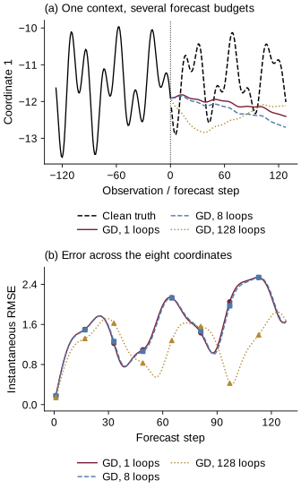
Do More Test-Time Steps Make Better Forecasts?

Imagine receiving a short recording of a moving pattern. You do not know the equation that produced it. The task is to predict the next part of the recording, and the model is allowed to think for a little longer before answering. Should more computation make the forecast more accurate?

The appealing answer is yes: another iteration should refine the estimate of the dynamics. Yet an iteration can also make the model more faithful to a noisy measurement, an uninformative direction, or an imperfect surrogate objective. Its progress meter may go down while its forecast error goes up. A numerical optimizer does not know which part of its target is physical signal unless that distinction is supplied by the model and the data.

This is a hypothetical forecasting setting, not a weather or engineering deployment. The experiments below use stable affine systems and a periodic advection–diffusion equation whose clean solutions can be evaluated independently. Their simplicity is useful: when a forecast fails, the uncertainty is not whether the reference simulation secretly failed first.

The starting point is Lai and colleagues’ Test-Time Forecasting, a 2026 preprint connecting recurrent linear attention, dynamical-system regression and small models that adapt during inference [1]. Here the contribution is a small-scale independent reimplementation, not a full reproduction of the authors’ datasets, optimizer or numerical results. DMD, test-time adaptation, Fourier operators and attention’s connection with gradient descent all have established predecessors [2–10]. The question is narrower: what does extra computation buy under a declared observation model and a fixed evaluation rule?

The answer was conditional. Extra updates helped several declared forecasts, yet better context fit and better future prediction sometimes separated. A squared-normalization LDS model was usable where the source-rule variant failed; pretrained Fourier starts improved on identity, but clean direct least squares was substantially more accurate. None establishes a universal law of test-time scaling.

What is the model allowed to look at?

A context is a sequence of observations already available when the prediction is issued. The future is a separate sequence. This sounds obvious, but a forecasting experiment can quietly cross the boundary in several ways: selecting the best iteration after seeing future error, smoothing observations with later truth, or allowing a rolling predictor to use the real next state instead of its own last prediction.

Write the observed context as a matrix $U$ whose rows are successive states. The final row is the latest observation, not the first point of the future. During autoregressive rollout, each predicted state enters the next context. Errors can therefore change not only the current answer but also the information used to produce subsequent answers. A one-step success is useful evidence, but it does not establish a reliable 128-step forecast.

The experiments keep that separation explicit. All methods see the same initial conditions and the same corrupted context. They start from its final noisy observation and are scored against a clean future that is never returned to the learner. The true equilibrium of an affine system is likewise available to the evaluator, not to preprocessing. Validation trajectories can choose a regularization strength or stopping rule; test futures cannot.

A fixed held-out linear-system trajectory compares analytic gradient-descent forecasts at one, eight and 128 iterations, with error across eight coordinates. — Figure 1. Predeclared held-out system LDS55, trajectory zero, clean context. (a) Coordinate one and analytic GD forecasts using 1, 8 and 128 updates; the vertical line separates context from future. (b) Instantaneous RMSE across all eight coordinates. This is a fixed illustration, not a best-case selection or a learned-model result. Extra updates use the same observations, and sliding forecasts append predictions only.

Why start with a linear regression?

Dynamic mode decomposition, or DMD, provides a useful first answer to the question “what propagation rule fits these successive snapshots?” It is not a claim that every physical system is linear. It is a particular regression whose geometry can be inspected and whose solution can be computed by independent methods [2,3].

Let $X$ contain all but the last context state and let $Y$ contain all but the first. A row-wise linear predictor is a matrix $B$ such that $XB$ approximates $Y$ . Its squared residual objective is

L(B)=\frac12\|XB-Y\|_F^2.

The Frobenius norm adds the squared discrepancies across snapshots and channels. Fitting this objective asks for a good account of transitions already observed. It does not directly optimize a long future. The least-squares solution can be represented using a pseudoinverse, but whether that solution identifies a unique propagator depends on which directions the context excites.

A short recording of motion on a line does not identify how an operator behaves away from that line. More snapshots of exactly the same motion may reduce uncertainty along it without adding the missing directions. This is a rank question, not merely a training-budget question. Tu and colleagues’ discussion of linear consistency makes such limitations part of DMD’s interpretation rather than a peripheral numerical nuisance [3].

Affine dynamics add a constant forcing. They can be represented linearly by adjoining a constant coordinate. That extra coordinate must be handled consistently when estimating the operator and when checking rank. Otherwise a bias term can masquerade as a dynamical mode, or a purported eight-dimensional spectral recovery can omit the part that makes the system affine.

What does another gradient step actually change?

For the declared loss, gradient descent takes the form

B_{\ell+1}=B_\ell-\eta X^\top(XB_\ell-Y).

The index $\ell$ counts optimization steps, not physical time. An additional step moves the fitted propagator using the same snapshot pairs. It does not advance the physical system or add a new observation. Confusing these two clocks makes “more depth” sound like “more knowledge”.

The singular values of $X$ reveal which directions move quickly. Along a direction with singular value $\sigma$ , the corresponding error is multiplied by $1-\eta\sigma^2$ . A large singular value creates a steep direction; a small one creates a slow direction. A step that is comfortable for one direction may overshoot another. For nonzero $X$ , the standard contraction condition on nonzero singular directions is

0<\eta<\frac{2}{\|X\|_2^2}.

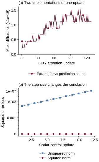
This squared norm matters. Rescaling the data changes the curvature quadratically. A denominator proportional only to the unsquared norm does not preserve that scaling. Appendix B.2 of the target v1 uses an unsquared-norm justification; this study retains that rule as a diagnostic and separately evaluates a squared-Frobenius normalization. The local algebraic mismatch does not establish that all the original experiments are invalid.

When $X=0$ , division by a norm is not a meaningful step-size rule. The gradient is zero and the objective contains no information about $B$ . When $X$ is rank deficient, every component in its null space also remains invisible. With $P_0$ the orthogonal projector onto that null space,

P_0B_\ell=P_0B_0.

Thus convergence of fitted values is not the same as convergence to a unique parameter matrix. A zero initialization can select a minimum-norm solution, but a different initialization retains a different invisible component. Reporting “the iterations reached the pseudoinverse” without specifying initialization would erase exactly the ambiguity that the experiment should expose.

Independent gradient and prediction-space updates are checked alongside the effect of squared versus unsquared step-size normalization. — Figure 2. Exact regression controls, separate from learned-model performance. Matched parameter-space and prediction-space iterates test the algebraic identity. Step-size controls use the same data and initialization; an unstable source-rule diagnostic is retained rather than repaired by clipping. Null-space and zero-input checks establish the limits of parameter recovery.

Where does linear attention enter the calculation?

Let $S_-$ select all but the final context row, so $X=S_-U$ , and define prediction-space iterates $Z_\ell=UB_\ell$ . Multiplying the parameter update by the complete context gives

Z_{\ell+1}=Z_\ell-\eta UX^\top(S_-Z_\ell-Y).

The matrix product has the form of linear attention: a query–key product followed by multiplication by values. The “values” here are a residual, and the shift in time is part of the construction. It is an exact relationship for this regression with these variables and matching initialization. It is not the statement that an arbitrary Transformer must perform DMD.

The distinction matters because learning can change the relationship. Independent projections of queries, keys, values, recurrent state and output can make a more useful predictor while breaking the identity with the original quadratic optimizer. A learned encoder can change which directions are emphasized. A learned temporal filter can change which pairs are compared. Once those choices are free, their behaviour needs empirical evidence rather than an inherited convergence label.

The general idea that linear attention can implement gradient-based regression predates this study [6]. EDMD likewise predates it: selected features can turn a nonlinear prediction problem into a linear regression in a richer representation [4]. Such lifting does not remove approximation error, poor conditioning or distribution shift. Convergence results for EDMD have explicit sampling and function-space assumptions; they cannot be substituted for a guarantee on a finite noisy context with trained projections [5].

The appeal of the construction is therefore not that it makes forecasting automatic. It makes part of the computation interpretable. We can ask which residual it reduces, which directions the context informs and which assumptions cease to hold after training.

What did the 620-parameter model learn?

The linear-system case reconstructs the small recurrent architecture rather than replacing it with a large generic network. An 8→9 affine encoder and a 9→8 decoder contribute 81 and 80 parameters. Five 9×9 Q/K/V/Z/O projections contribute 405, and the two-point temporal filters contribute 54. The total is 620. Parameter-count and time-alignment checks are important: a model with the right name but a different filter convention is not the same numerical question.

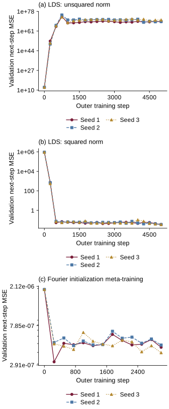
There are two separately trained normalization variants. Each uses three training seeds, 5,000 outer steps, batches of 16 and 35 recurrent updates during training. The outer optimizer is AdamW, with maximum learning rate $5\times10^{-4}$ , weight decay $10^{-3}$ , gradient-norm clipping at one and a linear decay over the final tenth of training. Checkpoints are selected using validation data.

These budgets are substantially smaller than the source study, and AdamW replaces its SOAP optimizer. That is a declared independent choice, not a controlled comparison of AdamW against SOAP. If the smaller run fails to recover a reported effect, several explanations remain: the training budget, optimizer, data, numerical implementation and the effect itself. Independent tests can eliminate some implementation errors; they cannot turn the remaining alternatives into a single causal conclusion.

All six LDS fits completed 5,000 steps. Among saved trained checkpoints, the source-rule seeds’ best validation MSEs nevertheless ranged from $6.32\times10^{49}$ to $2.17\times10^{52}$ ; the squared variants ranged from 0.0347852 to 0.0357830. Selection covered steps 250–5,000, excluding the initial step-zero diagnostic; the source-rule seeds selected step 250 despite a better initial diagnostic. Completion and useful learning were plainly different. This smaller AdamW outcome does not automatically refute the original SOAP-trained models.

Validation losses across three training seeds compare the two recurrent LDS normalization variants and Fourier initialization meta-training. — Figure 3. Validation next-step MSE across three training seeds: (a) LDS unsquared norm, (b) LDS squared norm, (c) Fourier meta-training. Traces are seeds, not confidence intervals. LDS checkpoint selection excludes the initial diagnostic and covers steps 250–5,000; source-rule seeds select 250. AD considers step zero plus 250–3,000, but all selected AD checkpoints are trained, using single-trajectory, 32-update validation. No test futures select checkpoints. Arithmetic completion does not imply a useful predictor.

Why use systems that eventually settle down?

The reference systems obey

\dot x=Ax+b,\qquad x_*=-A^{-1}b.

Their matrices are stable and contain two decaying oscillations plus four nonoscillatory decaying modes. The exact solution can be expressed as

x(t)=x_*+e^{At}(x(0)-x_*).

The equilibrium is a fixed offset; the changing part contains the dynamics. A forecast can look excellent in raw relative error simply because it stays near a large equilibrium while missing the smaller oscillation. We therefore report both raw error and error normalized by the equilibrium-centered clean motion. Centering is an evaluation lens, not an extra equilibrium oracle given to the model.

The candidate pool and frequency-separation rule are fixed before training. Of the accepted candidates, 56 systems are split into 32 training, eight validation and 16 entirely held-out systems. Each training system supplies 64 training trajectories and eight separate ID test trajectories; each validation or held-out system supplies eight. Every clean trajectory has 2,048 equally spaced points on $0\le t\le100$ . The evaluated context and future each contain 128 points.

The entirely held-out systems still come from the same generating distribution. This is held-out system generalisation, not transfer to another physical law. The PDE parameter split later is a different type of extrapolation. Calling both “OOD” without explaining their construction would hide a substantial difference in difficulty.

Which baseline is allowed to win?

Persistence repeats the latest observation. SVD-DMD solves a least-squares propagation problem directly. Ridge-DMD stabilizes weak directions through a validation-selected penalty. Total-DMD treats errors in both snapshot blocks rather than pretending that only the response is corrupted. Analytic GD-DMD exposes the effect of stopping an iterative solution early. The two learned recurrent variants then ask whether training changes that behaviour usefully.

The methods need not have equal costs to be informative. A direct solver can provide a reference even when it is not the intended deployment mechanism. But cost must be reported rather than erased by counting only loops. One loop through a 620-parameter recurrence and one SVD are different operations. Training cost is also separate from inference cost; a cheap forecast may depend on a substantial preparation stage.

Classical noise-aware DMD work motivates these controls [7,8]. It does not say that total-DMD must dominate here. Finite data, regularization, a strong offset and numerical rank can all matter. The comparison must permit persistence or a simple direct solution to be competitive, and must permit the learned model to fail.

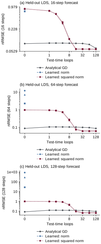
For clean held-out LDS at 128 updates, the squared-model seed medians were 0.0692118, 0.0636388 and 0.0722670, each over 128 successful trajectories; persistence was 0.0855933. The centered medians were much less reassuring: 0.881126, 0.830133 and 0.876996. Ridge-DMD achieved a raw median $1.6307\times10^{-5}$ with no failures. Ordinary DMD’s $3.3437\times10^{-6}$ median covered only 70 of 128 trajectories, with 58 failures. All 128 held-out trajectories failed at this budget for each source-rule seed. Accuracy without its denominator would tell the wrong story.

Clean held-out linear-system errors at 16, 64 and 128 forecast steps compare analytic GD and both learned recurrent variants across loop counts. — Figure 4. Clean, entirely held-out LDS forecasts at horizons (a) 16, (b) 64 and (c) 128, across the nine declared loop counts. Lines compare analytic GD and the two learned recurrent normalizations; different markers identify training seeds. Each point is a conditional median of successful finite trajectories, not a confidence interval. Failed runs remain in counts rather than becoming zero error; direct-solver baselines are reported separately.

Does a smaller context residual mean better dynamics?

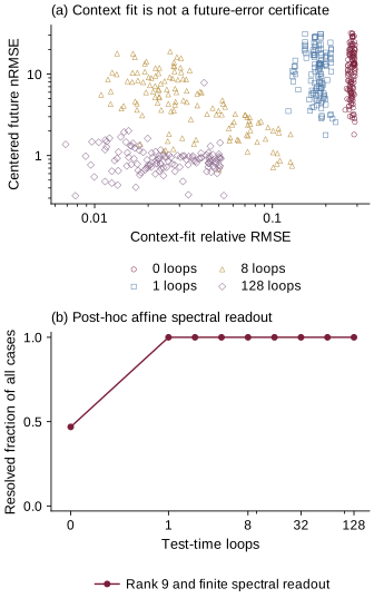
There are at least three different achievements: reducing the residual on observed transitions, forecasting unobserved transitions and estimating a dynamical operator. They can coincide in a well-conditioned, correctly specified and nearly noiseless problem. They need not coincide in the problems that make forecasting interesting.

To make this distinction measurable, the study records context residual, one-step error and longer-horizon nRMSE. It also fits an affine DMD operator to a predicted physical trajectory after forecasting. That spectral readout is a diagnostic of the produced trajectory, not a claim to have extracted a unique internal operator from the attention weights.

The fitted diagnostic uses the same relative SVD cutoff, $10^{-12}$ , and reports its effective rank. An augmented affine fit needs sufficient rank to support its spectral comparison. If it does not have that information, the readout is marked unresolved; missing modes are not manufactured to make a complete eigenvalue plot.

Even a full-rank readout deserves caution. Eigenvalues near the unit circle may be difficult to distinguish over a short window. A small eigenvalue discrepancy does not by itself protect every initial condition or every long rollout. Conversely, a model can produce a useful finite-horizon trajectory while its post-hoc operator is not a faithful physical identification. The error plots and spectral plots answer related but different questions.

From eight to 128 updates, 92 of 4,608 finite LDS pairs had a lower context residual but higher future error. AD had 2,084 such cases among 6,720 finite pairs—all from random initialization, none from identity or pretrained starts. Some occurred without observation noise; these counts do not isolate universal “noise overfitting”. They pool declared regimes descriptively, not independent statistical replications. For the first squared LDS seed at 5% noise, resolved rank-nine readouts increased from 60/128 at zero updates to 128/128 at 128 updates, but full rank still did not guarantee accurate dynamics.

Context residual is compared with clean forecast error and a post-hoc spectral diagnostic, with low-rank readouts left unresolved. — Figure 5. First squared-norm training seed on held-out LDS with 5% training-context fluctuation-RMS noise. (a) Context residual versus centered 128-step error at 0, 1, 8 and 128 updates, for positive finite successful values. (b) Fraction of all cases with rank-nine, finite post-hoc affine spectral readouts. The relative SVD cutoff is 10 to the power minus 12; full rank is a prerequisite, not proof of accurate identification. True equilibrium is used only in scoring.

What changes when the state is a field?

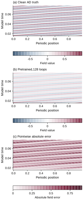
The second case is a periodic field transported and smoothed by

u_t+c\,u_x=\nu u_{xx}.

Advection shifts a pattern; diffusion attenuates its fine structure. On a periodic domain, Fourier modes separate those actions. For domain length one and $\kappa_k=2\pi k$ , the exact sampled propagator is

\widehat u_k(t+\Delta t)=e^{-(\nu\kappa_k^2+ic\kappa_k)\Delta t}\widehat u_k(t).

The multiplier’s magnitude describes decay and its phase describes translation. There is no discretization of a spatial derivative in this reference: the Fourier formula generates float64 truth directly. Grid comparisons at 128, 256 and 512 points check that the implementation respects the band-limited field rather than rewarding a particular spatial mesh.

The main grid has 256 points and retains seven Fourier modes, with initial signal only at $|k|\le6$ . The initial field has zero mean and maximum absolute value one. The sampling interval is $1/2048$ , context length 32 and forecast length 128. These are declared choices for the independent experiment, not recovered undocumented settings from the source.

Twenty parameter pairs follow $q=j/19$ , $c=100^q$ and $\nu=10^{-3-3q}$ . The first ten pairs form the ID region and the remaining ten are entirely held out for parameter extrapolation. For each ID pair there are 32 training, eight validation and 16 test trajectories; each held-out pair has 16 test trajectories. Because speed and diffusivity change together, the benchmark does not isolate their individual effects.

An advection–diffusion field and its forecast are compared through the true field, predicted field and spatially resolved error. — Figure 6. Predeclared AD19, trajectory zero, first training seed and clean context: (a) analytic truth, (b) pretrained adapter after 128 updates and (c) absolute pointwise error. Truth and prediction share a symmetric colour scale covering both fields' finite amplitudes; error has its own nonnegative scale. All 128 future frames are displayed, but only every fourth spatial point (64 of 256). Full fields are saved and scored. Model time is not calibrated seconds; the fixed illustration is not selected by accuracy.

Why can a tiny Fourier model be useful?

A seven-mode adapter is small because the reference equation is diagonal in Fourier space. It is not discovering a general nonlinear PDE solver. A local scalar connection and complex spectral weights define effective multipliers

G_k=W_k+w_{\mathrm{loc}}.

The encoder and decoder are fixed at one. Seven complex weights and one real local weight put 15 real quantities into the optimizer; including the two fixed scalar maps gives 17 stored quantities. Neither count is a count of identifiable physical degrees of freedom. A real inverse transform cannot see every stored complex component, and only modes carrying signal can constrain their multiplier.

On clean band-limited inputs there is also a gauge ambiguity: adding the same real amount to the local connection while subtracting it from every retained spectral weight leaves the retained-mode multipliers unchanged. It changes the gain on unretained modes, so this is not an invariance of the complete full-spectrum operator or necessarily of noisy data. Individual weights are therefore not independent physical parameters even in exact arithmetic. The physically relevant object is the combined multiplier on an excited mode, followed by a further question about whether its phase determines a unique speed.

Fourier least squares supplies a direct comparison. For a mode with nonzero observed power, its best complex multiplier is obtained from paired Fourier coefficients. Parseval’s identity connects this spectral residual to the spatial squared residual, provided the transform normalization and one-sided weighting are handled consistently. The independent spectral and spatial loss checks prevent a missing factor for positive-frequency pairs from changing the adaptation problem.

A direct optimum does not eliminate noisy-input bias. The observed coefficient appears in both the regressor and the successor relation, so a lower residual can still correspond to a worse clean multiplier. It does distinguish slow optimization from the information and objective limitations that remain even after optimization finishes.

What does pretraining contribute to adaptation?

Identity, random and pretrained initializations begin the same inner AdamW procedure in the main comparison. Its learning rate is 0.01, its betas are $(0.85,0.999)$ and its weight decay is zero. The source’s different random-initialization preset is retained only as a separately labelled diagnostic. Otherwise an apparent initialization advantage could instead be an optimizer-setting advantage.

Pretraining learns a starting point, not a new PDE parameter for every test example. Three seeds each run 3,000 outer steps with eight trajectories from one system per batch. The same fast weights are adapted jointly to those eight trajectories. Evaluation adapts to just one trajectory, and resets both initialization and optimizer moments for every independent test. Carrying moments between examples would introduce an undeclared stream of extra information.

The inner loss is mean space–time MSE on the context. The outer loss is the next-step prediction error. The computation differentiates through the complete AdamW adaptation, including its moment state, instead of detaching the learned initialization or truncating the meta-gradient. Independent finite-difference and automatic-differentiation controls check this path. Correct differentiation establishes what was optimized; it does not establish that the learned initialization is beneficial.

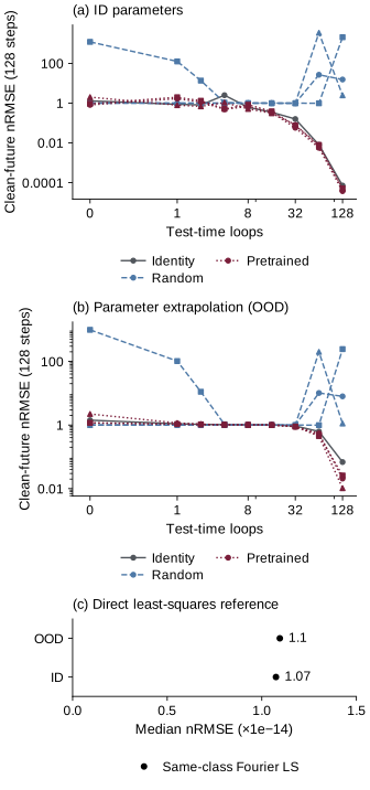
At 128 updates, each clean parameter-extrapolation summary contains 160 successful finite trajectories per initialization/seed. Identity’s median 128-step nRMSE is 0.0683804; the three pretrained seeds give 0.0207394, 0.0258472 and 0.0103202. Pretraining improves these medians relative to identity, but the direct same-class Fourier least-squares median is $1.0954\times10^{-14}$ . In this clean, correctly specified example, an excellent direct fit remains a much stronger reference than a comparison between learned initializations alone.

Median improvement is not uniformly accurate forecasting. The pretrained seeds’ empirical 75th-percentile errors are 0.527004, 0.491229 and 0.482726. These describe spread across the 160 trajectories, not confidence intervals. The fixed extreme-parameter illustration therefore belongs beside the medians; a typical-case number alone would hide substantial poor forecasts.

Random initialization gives medians 7.9693, 244.0531 and 1.1153 under the same main preset. All 160 trajectories per seed remain below the declared relative-blowup failure threshold of one million. They are poor finite forecasts, not numerical failures. Treating them as failed and dropping them would erase a major negative result. These numbers describe the small independent study, not a controlled refutation of the source’s different random preset or training procedure.

Identity, random and pretrained Fourier initializations use a matched inner optimizer, with a separate same-class least-squares reference panel. — Figure 7. Clean AD 128-step forecasts: (a) ID and (b) parameter extrapolation compare identity, random and pretrained starts using the same AdamW preset; (c) same-class Fourier least squares is shown separately near 10 to the power minus 14. Its ID/OOD summaries each contain 160 successful trajectories, no failures. Seed-specific adaptive curves are conditional medians, not uncertainty bands. Tests reset moments and use one trajectory, unlike eight-trajectory pretraining batches. The source's special random preset is not part of these matched curves.

How does noise change the stopping problem?

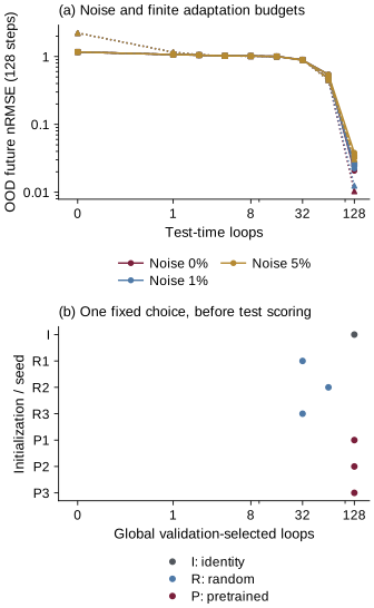
The noise levels are 0%, 1% and 5% of training-context fluctuation RMS, not of total state or field magnitude. Each training trajectory has its own temporal context mean removed first: scales are per channel for LDS, while AD centers each spatial location before aggregating. No true equilibrium is used to set the noise. Every method receives the same realization. This pairing makes a difference between methods easier to interpret, but it does not create extra independent repetitions. In particular, thousands of scored time points are not thousands of independent training runs.

Early iterations can act as an implicit regularizer: well-excited directions move before poorly informed ones. Later iterations may improve clean forecasting, or may fit errors that are not predictive of the clean future. Neither direction is assumed. Noise-aware DMD, ridge regularization and early stopping are different responses to this problem, and a matched comparison can reveal where their effects overlap.

A stopping rule selected on validation data can be used without test labels. The best iteration chosen retrospectively from a test future cannot. That oracle curve can be a helpful diagnostic of remaining headroom, but it is not a deployable predictor. The article keeps those categories separate rather than presenting a hindsight optimum as the outcome of an online decision.

With 5% fluctuation-RMS observation noise and 128 updates, identity’s held-out median rises to 0.0796871, while the three pretrained medians are 0.0381882, 0.0334018 and 0.0306020; each again contains 160 successful finite trajectories. Same-class least squares gives 0.0183728. Its near-roundoff clean result no longer implies a near-roundoff noisy forecast: fitting the available observations does not recover information erased by their corruption.

The global validation rule selects 128 updates for identity and all three pretrained seeds, and 32, 64 and 32 for the random seeds. These choices are shared across the declared noise levels, not tuned separately on each test regime. The 128-update random comparisons above describe a fixed budget, not those selected policies. No hindsight test optimum is promoted to a usable stopping rule.

Clean-future forecasting at zero, one and five percent observation noise is compared across adaptation steps and validation-selected stopping. — Figure 8. (a) Pretrained AD adapters on held-out parameters at 0%, 1% and 5% noise, with separate seed traces. Percentages use centered training-context fluctuation RMS, not total field magnitude. (b) One global loop choice per initialization/seed, selected across all ID validation trajectories and all declared noise levels before test scoring. These are validation choices, not hindsight optima from test futures. Conditional medians exclude failed cases, whose counts remain available.

Can a perfect forecast still identify the wrong speed?

For a Fourier multiplier with nonzero magnitude, one might estimate speed and diffusion from

c_k=-\frac{\arg G_k}{\kappa_k\Delta t},\qquad \nu_k=-\frac{\log|G_k|}{\kappa_k^2\Delta t}.

The second expression uses a magnitude, but the first uses an angle returned modulo a full turn. A phase is not automatically an unwrapped physical displacement. A fast pattern can travel around the periodic domain and look like a slower one at the sampling instants.

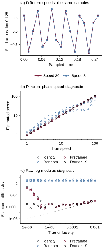
An exact control makes this visible without optimization. Hold the initial field and diffusion fixed, set $\Delta t=1/64$ , and compare speeds 20 and 84. Their difference moves the field by one complete domain length between observations. For every integer mode,

e^{-i2\pi k(84-20)/64}=1.

The two sampled propagators are identical. Their fields can differ between observations, but no algorithm using only those samples can distinguish them. More adaptation, a better initialization or a lower training residual cannot supply the missing temporal information.

This control is not the main experiment’s sampling regime and is not evidence that its speeds must be wrong. It demonstrates the extra assumption hidden inside a physical parameter interpretation. A finer sampling rate or a justified speed range can remove the ambiguity; an arbitrarily confident fitted multiplier cannot. Prediction and identification remain distinct even when a model class exactly contains the true sampled propagator.

Periodic fields transported at speeds 20 and 84 coincide at samples spaced one sixty-fourth apart despite different motion between samples. — Figure 9. (a) First 17 of 160 samples in the exact aliasing control: speeds 20 and 84, common sine initial field, diffusivity 0.0001 and interval 1/64; curves intentionally overlap. (b,c) Principal-phase speed and raw log-modulus diffusivity diagnostics on all 20 main parameter pairs with 5% noise, using global validation-selected loops. Seed-specific medians include successful finite cases only. Raw diffusivity estimates are not clipped; the symmetric-log axis permits negative values. The control is separate from main 1/2048 sampling.

How much computation is an extra step worth?

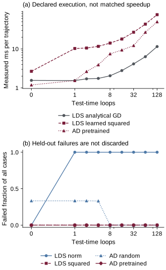
An adaptation curve should be read together with a cost and failure curve. A method that gains a little accuracy at 128 iterations may be useful when inference time is available; the same method may be inappropriate when a direct solver attains the target sooner. A model that occasionally diverges cannot be evaluated only on its attractive completed forecasts.

The evaluation records actual adaptation work and training work separately. Independent test examples reset state, and timing is not expected to reproduce bit for bit. Two formal runs execute concurrently through four one-thread family workers on a shared CPU. These timings measure the audit’s work, not clean isolated inference latency. Scientific outputs are compared under the same source and configuration; runtime is saved separately. This distinction prevents scientific agreement from being advertised as a hardware-independent speedup or latency guarantee.

Nonfinite values and large relative blowups are retained with their failure categories. No forecast is clipped back to a plausible amplitude, and no eigenvalue is silently projected into a stable region. Those interventions could be legitimate different methods, but they would change this question. Finite-case accuracy summaries therefore state how many cases they include and sit alongside failure counts.

The flags use case-specific scales. LDS flags nonfinite forecasts or per-step eight-channel RMS above one million times observed-context RMS. AD flags nonfinite forecasts/gains or pointwise maximum absolute forecast above one million times clean-future RMS. That truth-derived AD scale is scoring information only, never adaptation input. These diagnostic cutoffs are not physical safety standards; cross-case failure fractions do not measure identically normalized risk, and passing a cutoff does not establish useful accuracy.

Two complete runs agreed on their scientific outputs. The LDS table retains 77,184 method–budget records, including 28,761 failures; AD retains 62,400, including 2,558. These are correlated evaluation records, not independent trials. Each shared-CPU run took about 23.3 minutes. Independently implemented GD/attention iterates differed by at most $1.55\times10^{-15}$ ; such implementation checks support the comparison, not a learned-model accuracy guarantee.

Forecast accuracy, measured adaptation cost and retained failures are presented together rather than ranking methods by loop count alone. — Figure 10. (a) Measured audit work for selected GD, first-seed squared LDS and first-seed pretrained AD: LDS divides batched-eight forecasts by eight; AD uses fresh one-trajectory fit-and-rollout probes. Two formal runs share a CPU through four one-thread family workers, so this is not an isolated latency benchmark or a matched speedup. (b) Held-out failure fractions at 5% noise retain all cases; three learned seeds are pooled for descriptive counts only, not population uncertainty. Training cost and scientific repeatability are separate.

What this comparison can—and cannot—settle

The two cases deliberately expose mechanisms rather than cover the world of forecasting. Stable affine systems do not test chaos, changing laws or hidden inputs. A diagonal linear Fourier equation does not test nonlinear mode transfer. The correlated PDE parameter sweep is useful for controlled extrapolation, but cannot establish robustness to independent changes in every physical coefficient.

Only three training seeds are available for each learned setting. Their variation should be displayed, not buried in a pooled standard error that treats all trajectories as independent model replications. The finite collection of systems likewise supports benchmark comparisons, not a population-level reliability estimate for an unknown deployment environment.

The strongest exact statement is about a specific quadratic update and a specific sampling counterexample. The learned model comparisons are numerical evidence under a frozen protocol. A passing gradient test, matching parameter count or repeated run supports implementation reliability; it does not certify a generalization theorem. Those distinctions let a disappointing learned-model result remain informative instead of being hidden by a stronger story.

Test-time training itself is established background [9]. The practical issue is what adaptation is allowed to optimize, how its information relates to the forecasting target and when its costs are justified. In a correctly specified clean regression, extra work can reduce genuine numerical error. In a noisy or unidentifiable problem, optimization can finish without resolving the scientifically important uncertainty.

Conclusion

More computation was useful in specific settings, not a substitute for a suitable objective, initialization or observation design. The verified study supports a bounded comparison and preserves its negative outcomes; it does not claim a new forecasting principle or a quantitative reproduction of the original paper.

The outcomes reinforce a central distinction: fitting an observed context, predicting a clean future and identifying a physical law are not interchangeable achievements. More test-time computation changes the first directly. It improves the others only through assumptions about the objective, the observations, the model class and the information carried by the context.

Before asking a forecasting model to think longer, ask what its next step is trying to solve. Is the residual still telling it something about dynamics? Can the context distinguish the parameters being reported? Was the stopping point selected without seeing the answer? Those questions turn a smooth “more compute” curve into an interpretable research result.

See the project overview for the two-case design and the boundaries of this independent study.

References

Lai, Quinn, Bao and Gilpin. Test-Time Forecasting: Recurrent Depth Enables In-Context Dynamics Prediction (2026), v1. Primary preprint.
Schmid. Dynamic mode decomposition of numerical and experimental data (2010). Published paper.
Tu, Rowley, Luchtenburg, Brunton and Kutz. On Dynamic Mode Decomposition: Theory and Applications (2014). Published paper.
Williams, Kevrekidis and Rowley. A Data-Driven Approximation of the Koopman Operator: Extending Dynamic Mode Decomposition (2015). Published paper.
Korda and Mezić. On Convergence of Extended Dynamic Mode Decomposition to the Koopman Operator (2018). Published paper.
von Oswald and colleagues. Transformers Learn In-Context by Gradient Descent (2023). Primary conference paper.
Hemati, Rowley, Deem and Cattafesta. De-Biasing the Dynamic Mode Decomposition for Applied Koopman Spectral Analysis (2015 preprint, 2017 journal). Primary preprint.
Dawson, Hemati, Williams and Rowley. Characterizing and correcting for the effect of sensor noise in the dynamic mode decomposition (2016). Published paper.
Sun and colleagues. Test-Time Training with Self-Supervision for Generalization under Distribution Shifts (2020). Primary conference paper.
Li and colleagues. Fourier Neural Operator for Parametric Partial Differential Equations (2021). Primary preprint.