
Imagine releasing a small quantity of dye into a network of connected tanks. A sensor near the outlet should trigger an alarm if too much material accumulates there during the next few hours. Two proposed routing designs have identical removal rates, identical injected mass and exactly the same eigenvalues. An asymptotic stability check gives them the same answer. Should the monitoring decision also be the same?
Not necessarily. The route taken by the material determines when it reaches the sensor, while removal continues throughout the journey. A short route may concentrate material at the target early enough to cross a threshold. A longer route may spread arrival over time, leaving more opportunity for removal before the same target fills. Both networks eventually empty. Their equal long-run decay information does not settle the finite-time alarm.
This is a hypothetical transport experiment, not a calibrated pollution assessment. The state variables are nonnegative amounts in idealized compartments. The alarm threshold is a declared modeling choice, not a regulatory limit. That distinction matters because the mathematical counterexample is useful without pretending that it has established what a real monitoring authority should do.
The underlying ideas are established. Phase-type distributions describe transit through Markov stages; positive-system analysis preserves mass and signs; nonnormal dynamics explains why eigenvalues do not summarize every transient. Recent work by Bao and colleagues explicitly relates localized inputs and network transients to directed walks [1–4]. The useful contribution here is a narrower, verified comparison: when routing changes but those physical bookkeeping rules stay fixed, which calculations can resolve a particular finite-horizon threshold decision?
Nazerian and colleagues’ 2026 study of networks as open systems likewise makes the selection of input and output nodes explicit, using frequency response and the norm [5]. The present question is not whether network structure affects transfer. It is whether a specific occupancy peak exceeds a declared threshold before a deadline, and whether a bound can certify that answer under matched routing changes.
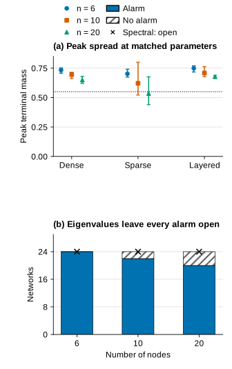
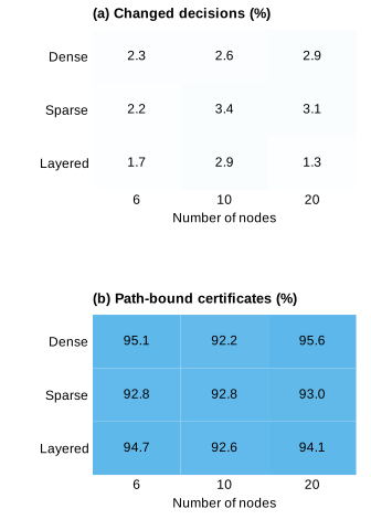
The held-out comparison found 172 changed alarms among 6,912 paired threshold queries, while 6,740 remained unchanged. The path-specific envelope certified 6,473 unchanged decisions; the basic norm bound certified 3,147. This is a controlled synthetic result, not a new transient theory or an estimate of real-world alarm prevalence.
What the sensor asks is not what stability asks
An eigenvalue describes an exponential rate associated with a linear system. For an autonomous model with all eigenvalues strictly in the left half-plane, perturbations eventually decay. This is an important conclusion. It rules out sustained exponential growth in the model. It does not specify how much of a localized release reaches a selected compartment before that decay becomes dominant.
A threshold monitor needs a specified input, output and interval: here, a unit release at one source, the amount stored at one sensor compartment, and a fixed horizon. Changing these choices can change the answer without changing the eigenvalues.
Let the amount vector be , with one coordinate for each compartment. We use a column convention: the off-diagonal entry transfers material from compartment to compartment . The total transfer out of a compartment is subtracted from its diagonal. Uniform removal acts everywhere at rate :
The sign condition makes , and therefore , a Metzler matrix. Its exponential maps nonnegative initial amounts to nonnegative amounts. The column-sum condition says that transfers redistribute material rather than creating it. Uniform removal then gives an exact balance equation, not an approximate conservation check:
For a unit release, the total surviving amount is exactly . No compartment can contain more than that total. An individual target can nevertheless fill while other compartments empty. An increasing sensor reading is not growth of total mass, and it need not be a numerical instability. It can be ordinary redistribution inside a decaying system.
Unlike unrestricted matrix-amplification examples, the comparison preserves nonnegative amounts and mass accounting. The transient difference survives physical restrictions rather than exploiting their absence.
The measured response from source to output , and its finite-horizon peak, are
An alarm means . Strict inequality is part of the definition: touching the threshold is not silently counted as exceeding it. Near equality, the computation must return uncertainty if its verified error cannot decide which side contains the true peak. A confident label is not more valuable than an honest unresolved case.
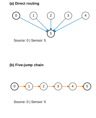
A spectrum can stay fixed while routes change
Concept guide · Assumption
A condition taken as given when constructing a model or argument; its conclusions depend on the relevant conditions holding.
In this article: The matched network construction uses acyclic routing, equal total transfer rates at transient nodes and uniform removal.
Common misconception: A plausible assumption is an observed fact.
Scope: These restrictions belong to this network construction. Other models and methods require their own assumptions; no single list applies to every analysis.
Consider six compartments ordered from source to terminal. Every edge points forward in this ordering, so there are no directed cycles. Each of the first five compartments transfers material onward at total rate . The final compartment has no transfer exit, although the same removal rate still applies there. Routing probabilities determine which later compartment receives each transfer.
Every such generator is lower triangular. Its diagonal contains five copies of and one copy of . Triangular matrices have their diagonal entries as eigenvalues. Consequently, changing any allowed routing probability preserves the entire eigenvalue multiset, not merely its largest real part:
The construction makes the limitation of eigenvalue-only screening unusually clean. The spectrum has no routing information available to separate the designs. A deterministic screening rule that receives only those eigenvalues and the common monitoring settings must return the same answer for all of them. If two valid routings have opposite alarms, such a rule cannot classify both correctly. This is an information limitation, not a failure to choose a clever enough spectral cutoff. Accordingly, the eigenvalue-only comparator reports asymptotic stability but abstains on the alarm; it is not assigned invented binary predictions.
Two extreme routings help explain why. In the direct design, material from the source jumps straight to the terminal. In the chain, it must make five successive transfers. The waiting time for each transfer is exponential with rate . The direct journey therefore has one waiting stage; the chain journey has five. Equal diagonal decay rates do not make these first-arrival times equal.
The direct-routing example is intentionally simple. It verifies the conventions, exposes the mechanism and supplies a closed-form reference. It is not a novel theorem or sufficient evidence for a new network-analysis method. A more useful benchmark must move beyond this pair, retain matched physical quantities and test whether conclusions survive held-out routing structures.
There is a further subtlety: equal eigenvalues do not imply equal eigenvectors, Jordan structure or transfer functions. The chain can introduce polynomial factors multiplying exponentials through repeated eigenvalues. Those factors encode delayed propagation. It is misleading to describe the comparison as if the networks had identical dynamics apart from one mysterious transient effect. They have identical spectral rates, but not identical dynamical maps.
Nonnormality is relevant background, but it is not an isolated causal treatment in this construction. A matrix is nonnormal when it fails to commute with its transpose. Structural nonnormality in networks is already well studied [9]. A commutator norm can summarize that property, yet it discards the identities of the release and sensor. Two networks can have similar diagnostic values and different source-to-sensor responses. Conversely, a changed diagnostic does not tell us which path caused a threshold reversal. The article therefore uses nonnormality as a diagnostic, not a calibrated alarm score.
Following material gives an independent exact answer
The same model has a probabilistic interpretation. Follow one representative unit of material. At a transient compartment it waits for an exponential clock of rate , then chooses its next compartment according to the routing probabilities. An independent removal clock of rate can eliminate it anywhere along the journey. Ensemble probabilities become compartment amounts because the model is linear.
Conditional on requiring exactly transfers to reach the terminal, the travel time is the sum of independent exponential waiting times. Its distribution is Erlang, a familiar phase-type distribution. Its cumulative distribution function is
This is a cumulative arrival probability before removal is applied. It is not the density of arrivals. Since the terminal retains transferred material except for uniform removal, the terminal occupancy for an -stage route is . The exponential factor accounts for survival through the whole elapsed time, including time spent at the terminal after arrival.
For a general forward routing network, let be the probability that the embedded jump chain first reaches the terminal in exactly transfers. These probabilities can be calculated by propagating probability mass one jump at a time and removing it from further propagation once it reaches the terminal. The exact response is then
The finite sum is exact for the declared acyclic, equal-holding-rate model. It is not a fitted approximation or a Monte Carlo envelope. The complete matrix exponential and the path calculation use different computational representations of the same dynamics, making them useful independent checks. Agreement should be reported as an error over declared test times, not as a vague visual overlap.
In this benchmark, every allowed transient node routes to a later node and the only terminal is the sensor, so eventual arrival without removal has probability one. In a more general network with alternative exits, the path weights need not sum to one. Renormalizing them would condition on successful arrival and exaggerate unconditional occupancy. That apparently harmless normalization would change the scientific question.
The equal exit-rate assumption is also doing real work. If different compartments have different holding rates, conditioning only on the number of jumps no longer gives a common Erlang law. One needs the actual sequence of rates or the general transient generator. Cycles introduce arbitrarily long walks, so the short finite path-length sum no longer applies. Phase-type methods remain available, but this article’s compact formula should not be carried into those settings unchanged [2,3].
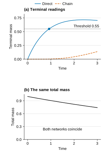
Why a longer route can avoid an early alarm
The direct and chain formulas differ only in the arrival distribution. A direct route places more probability on early arrival. A longer route delays and spreads arrival because several waiting stages must finish. Meanwhile, uniform removal reduces the surviving material. The peak therefore depends on a competition between arrival and loss, not simply on a decay eigenvalue.
For the one-stage route, differentiating gives an unrestricted peak time of . If that time lies beyond the monitoring horizon, the finite-horizon maximum is at the endpoint instead. This small detail illustrates why an infinite-time peak and a peak over the next three time units answer different questions. Neither should be substituted for the other when scoring an alarm.
For a multistage mixture, different arrival components can affect different portions of the response. A mean path length is useful for intuition but does not determine the whole curve. Two mixtures with the same mean can put different weight on very short and very long routes. An early threshold can react strongly to that short-route weight even when the mean remains unchanged.
Nor does a later arrival automatically imply a better design. A delayed response may fall outside one monitoring window and enter the next. A different sensor may sit directly on a formerly hidden route. A lower threshold may make both networks trigger. These are not failures of the mechanism; they reveal the need to specify the decision before comparing designs.
Each isospectral comparison fixes source, sensor, mass, removal and rates. Otherwise a lower peak might simply reflect less injected material or faster loss. New structures and parameter regimes test whether the mechanism extends beyond the dramatic introductory pair.
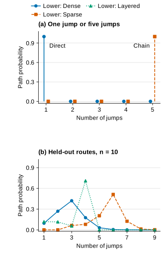
A reliable comparison needs more than a smooth curve
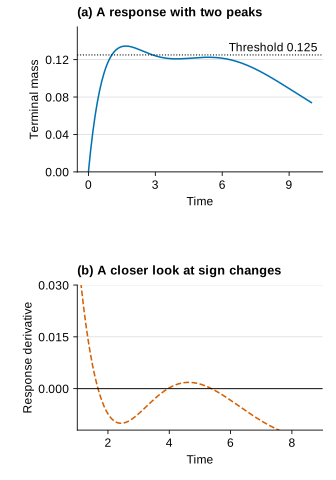
Calling a matrix exponential exact refers to the mathematical solution representation. Evaluating it on a computer still introduces floating-point error. Likewise, a closed-form path mixture does not make a sampled peak an exact continuous-time maximum. A narrow peak may lie between grid points, and a root finder can converge to one stationary point without proving that no other maximum exists.
Verification separates generator validation, independent response checks, and continuous-time peak decisions. Agreement at sampled times does not by itself control the maximum between them.
A time grid supplies a lower bound on the peak when the response values are enclosed reliably: the true peak cannot be smaller than every sampled value. To obtain an upper bound, the calculation needs control of what can happen between samples. A derivative bound can provide that control, while interval refinement focuses effort on time cells that could still contain a larger value. The resulting bracket is useful because it expresses what remains uncertain.
An alarm is verified when the lower peak bound exceeds the threshold. A no-alarm is verified when the upper peak bound is at most the threshold. If the threshold lies inside the bracket, the label remains unresolved until further permitted refinement succeeds. This tri-valued interpretation avoids turning a rounding convention into a scientific finding.
First crossing requires another layer of care. A peak above threshold establishes that a crossing exists when the initial value is below it and the response is continuous. It does not by itself give the earliest crossing time. A sparse sign-change search can miss an earlier excursion or a tangency. Crossing times should therefore be accompanied by their validation method and bracket, or left as numerical diagnostics rather than certified event times.
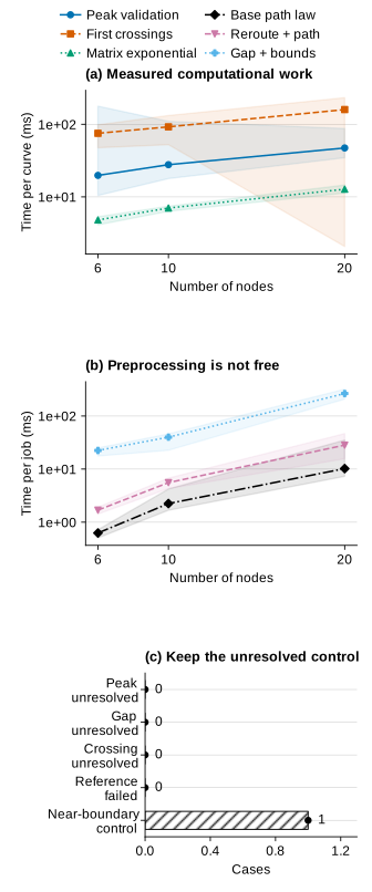
The complete evaluation enclosed all 2,880 continuous-time peaks and all 2,304 maximum response gaps to width at most . Earliest crossings, where present, were bracketed to width at most ; none of the formal threshold decisions or crossing checks remained unresolved. Independent matrix-exponential checks differed by at most . Routing coefficients were quantized first and then treated as the exact declared model. Two complete runs agreed on the scientific records. A separate, deliberately near-peak control exhausted refinement and remained unresolved; it was not silently added to, or removed from, the formal benchmark.
A bound answers a different question from a prediction
Concept guide · Robustness
The extent to which a specified result or level of performance survives specified changes in circumstances.
In this article: For two admitted routes, a valid response-difference bound below the nominal decision margin certifies that their alarms are the same.
Common misconception: An inconclusive certificate predicts failure, or robustness to one perturbation covers every perturbation.
Scope: This is a pairwise guarantee for the compared routes under the stated model assumptions. A whole-family guarantee would require a bound uniform over that declared family.
Suppose the nominal routing matrix is , but a revised or uncertain routing gives . Computing the exact response for both matrices can tell us whether their alarms differ. A robustness bound asks a broader question: is the nominal decision far enough from threshold that a declared perturbation cannot change it?
The starting point is Duhamel’s identity. The surrounding positive-system and Markov-chain perturbation theories are established [6–8]; the calculation here specializes them to the declared source, sensor and deadline:
This identity is valid without interpreting the matrices as transport. The useful simplification comes from the physical restrictions. The generators have common column sums , so their nonnegative propagators have column sums, and induced one-norm, equal to . Each column represents the surviving distribution from one unit release.
Applying the induced norm inside the integral gives a bound on the difference of any matched source-to-sensor responses. The two survival factors multiply to throughout the integration interval, yielding
For a finite horizon, maximize the right-hand side at . The peak difference is no larger than the uniform response difference, so
Why does this remain valid if the two peaks occur at different times? At every time the curves differ by at most the same uniform bound. Evaluating one curve at the maximizing time of the other gives one inequality; exchanging their roles gives the reverse inequality. No assumption of coincident peak times is needed.
The nominal decision margin is the distance from its peak to threshold. If that distance exceeds a valid perturbation bound, the revised peak cannot cross the threshold:
This implication is one-way. Failure of the inequality does not predict a changed alarm. It means that this particular certificate cannot settle the question. An exact comparison may still show identical alarms, or a sharper bound may certify them. Conflating an inconclusive certificate with an unsafe system would make the analysis systematically misleading.
Numerical enclosures belong inside the margin calculation. Use the closest verified endpoint of the nominal peak interval and a conservative upper endpoint of the bound, rather than distances between rounded point estimates. This may certify fewer cases, but does not hide numerical uncertainty inside a strict inequality.
A true inequality can still be practically empty
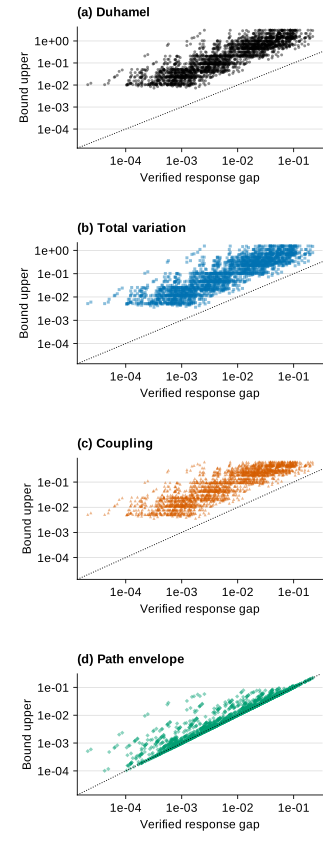
The induced one-norm bound is deliberately general. It pays for the largest changed column, regardless of whether the release reaches that column early enough to matter. It then allows every downstream effect to contribute in the most unfavorable direction at the selected sensor. These relaxations establish validity but discard much of the network geometry.
Consequently, the bound can be much larger than the actual peak difference. It can even exceed the maximum physically possible occupancy difference. That does not make the proof false. It makes the bound loose. The trivial physical range can tighten a numerical allowance, but it cannot manufacture enough information to certify a decision very close to threshold.
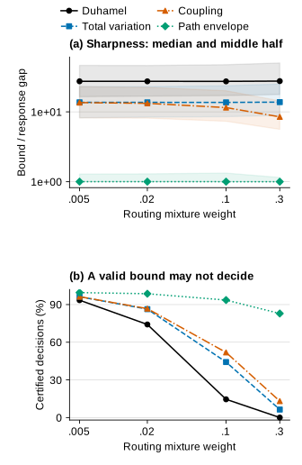
The right evaluation therefore includes sharpness and vacuity. Here sharpness compares a bound with the largest absolute response difference over the window; the difference between the two peaks is reported separately. Equal peak heights need not mean identical curves. Vacuity records whether the bound is too wide to certify the nominal alarm. A ratio is not always meaningful: if the verified response difference includes zero, the bound-to-difference ratio is left undefined. Such cases retain additive slack rather than an arbitrary denominator floor disguised as evidence.
Decision relevance also differs from absolute accuracy. A bound of one hundredth can be highly useful when the nominal peak is far from the threshold, and useless when the nominal peak lies one thousandth away. Conversely, a relatively loose bound can still settle a comfortable margin. The article therefore reports both response-scale sharpness and the actual decision coverage.
A further distinction is pointwise versus family-wide robustness. A bound comparing two known matrices does not automatically cover every physically allowed routing perturbation in a neighborhood. A family certificate needs a bound that is valid uniformly over that whole family. If the allowed changes are constrained by nonnegativity and outgoing probabilities summing to one, those constraints must remain part of the set being certified.
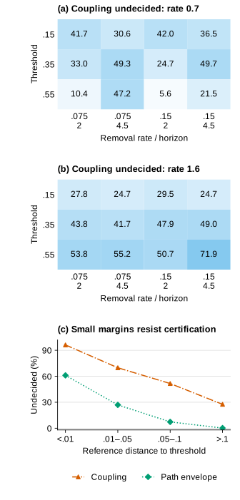
Across the 2,304 routing pairs, median bound-to-response-gap ratios were 27.38 for Duhamel, 13.69 for total variation, 11.47 for coupling and 1.00045 for the path envelope. No denominator was unresolved in this formal set. The path envelope was not uniformly sharp: its largest ratio was 48.50. The improved median therefore does not justify treating it as an exact response difference.
Keeping routing information can improve the question
The mass constraint already improves the global norm estimate. Each column of the difference between two conservative transfer generators sums to zero: its positive and negative parts have equal total mass. A selected output coordinate can distinguish those parts by at most the range of a probability-valued response. Writing the common perturbation size as , this gives the total-variation allowance
A coupling argument retains the idea that probability cannot separate repeatedly after it has already separated. Couple two trajectories until their routing first differs. A worst-case separation rate of gives
For small perturbations, expanding the exponential recovers the half-norm first-order behavior. For larger ones, the coupling allowance saturates instead of growing indefinitely with the norm. It is still a worst-case source-to-output allowance, not the exact difference for the chosen pair. Each time-dependent expression must be maximized over the same monitoring window before it bounds a peak difference.
In the acyclic equal-rate model, path probabilities permit a more specific calculation. Let , and let be the difference between the cumulative path-length probabilities up to . Both distributions sum to one. Substituting the Erlang formula and collecting equal powers yields
Replacing signed coefficients by their absolute values provides a path-specific envelope:
This bound retains which path-length probabilities changed, but loses cancellations between their contributions. If the cumulative differences have mixed signs, that loss can matter. If the two networks have identical path-length distributions, this envelope is zero even when their internal routes differ. The terminal output cannot distinguish every microscopic routing change.
Those possibilities should not be confused with a claim that a particular refinement is new. Probability distances, Markov coupling, induced input-output gains and path decompositions all have established theories. The benchmark asks how the selected bounds behave under fixed definitions and held-out tests. A useful application can be worthwhile without being a new theorem.
It is especially important to state what information a refined certificate receives. A calculation using the exact path distribution has more routing knowledge than eigenvalue-only screening. If it approaches the cost of an exact response evaluation, its role may be interpretation or repeated-query reuse rather than acceleration. Efficiency comparisons must count that preprocessing instead of presenting a cheap final formula as the whole algorithm.
The decision counts reveal how much those differences matter:
| Bound | Certified out of all 6,912 queries | Certified among 6,740 unchanged queries |
|---|---|---|
| Duhamel | 3,147 (45.53%) | 46.69% |
| Total variation | 4,029 (58.29%) | 59.78% |
| Coupling | 4,284 (61.98%) | 63.56% |
| Path envelope | 6,473 (93.65%) | 96.04% |
None of these certificates contradicted the verified decisions. The path envelope still left 439 queries inconclusive: all 172 actual reversals and 267 unchanged cases. It certifies agreement, not disagreement, and receives both path laws rather than only their spectra.
What should survive a held-out network test?
A single star–chain comparison establishes that eigenvalues are insufficient in principle. It does not establish how frequently the limitation matters in a broader routing family, how conservative a bound will be there, or whether an implementation behaves reliably away from the example that motivated it. Those require a split between development and evaluation.
The structure split holds out routing patterns, not merely new time points on a familiar curve. Development cases can reveal implementation mistakes and inform a predeclared comparison protocol. Held-out cases then ask whether that fixed protocol still works on different mixtures of short and long paths. Choosing the most dramatic held-out examples after seeing every outcome would turn the test into another demonstration set.
The parameter split serves a different purpose. Changing , , or changes the balance between travel, removal and monitoring. Within each comparison, the pair remains isospectral and physically matched. Across regimes, however, the common spectrum can change. Calling the entire sweep one isospectral population would conceal that distinction.
Dimensionless quantities clarify the regimes. The product measures how many transfer stages can typically occur before the window ends, while measures removal over that window. The ratio compares removal to onward transfer. Changing a time unit rescales rates and horizon together; it should not create a new physical conclusion. A useful sensitivity check respects that equivalence.
The threshold belongs to this evaluation design too. A threshold above every possible peak makes all cases no-alarm and creates trivial agreement. A threshold below almost every peak does the same for alarms. Neither demonstrates a good screen. The benchmark must retain both easy and difficult margins and state where its threshold settings came from, rather than adapting them to maximize one method’s apparent success.
Because these are constructed networks, success proportions describe the declared benchmark distribution. They are not estimates of failure prevalence in water infrastructure, epidemic transport or supply chains. Individual thresholds applied to the same network and parameter setting are also not independent field replicates. The meaningful unit of comparison must remain visible when reporting counts.
Evaluation used eight independent networks in each of nine family–size blocks: dense, sparse and skip-layered routing at 6, 10 and 20 nodes. Jump rates were 0.7 and 1.6, removal rates 0.075 and 0.15, and horizons 2 and 4.5. Each baseline was mixed with an alternate routing, , at weights 0.005, 0.02, 0.1 and 0.3; thresholds were 0.15, 0.35 and 0.55. Changed-query counts were 60, 67 and 45 in the three families respectively, out of 2,304 each. These are paired benchmark queries, not population failure rates.
Which failures are worth keeping?
An invariant decision is a useful negative result. Some routing changes may leave the terminal response almost unchanged. Others may change the peak but not cross the selected threshold. Both outcomes limit the story: routing matters to the transfer function, yet it does not force an alarm reversal for every pair or monitoring rule.
A vacuous certificate is another informative failure. It identifies a mismatch between the information retained by a bound and the question the sensor asks. If a norm-based estimate repeatedly fails far from threshold, it may be paying for physically unreachable or irrelevant changes. If it fails only at tiny margins, the difficulty may be intrinsic to the decision rather than evidence of a poor analysis.
Numerically unresolved decisions remain in the result set. Exhausting the declared refinement budget does not authorize inheriting the sign of a rounded nominal peak.
The same discipline applies to runtime. A formula may be quick after path weights have been computed, while a matrix exponential may serve several outputs at once. Reusing precomputed quantities changes the cost model. A meaningful report separates preprocessing, response evaluation, peak verification and certificate construction, and distinguishes operation counts from hardware-sensitive elapsed time.
The strongest conclusion may therefore be modest: a simple screen is incapable of distinguishing certain decisions, an exact route-aware calculation resolves them, and a rigorous margin succeeds only in part of the tested region. That is more useful than announcing that one method wins everywhere, especially when the failures explain which information each calculation discarded.
For repeated thresholds on one routing, precomputed response enclosures can be reused; for a new graph at every query, that advantage may disappear. The workload must be declared before announcing a speed advantage.
Independent references can be deliberately redundant during validation. Their combined work is not necessarily a future per-alarm cost, but belongs in the cost of producing this verified benchmark.
In one complete run, median per-curve times were 36.24 ms for peak verification, 89.45 ms for three-threshold crossing checks and 7.06 ms for the matrix-exponential reference. These components deliver different guarantees and exclude some preprocessing; dividing them is not an end-to-end speedup. The separate near-boundary control also shows why typical runtime cannot replace a refinement-budget policy.
What the model leaves outside
The compartment state is an amount. Interpreting it as concentration requires equal compartment volumes or an explicit volume normalization. Interpreting it as dose requires an exposure model. Interpreting it as a safe or unsafe engineering condition requires calibrated parameters, measurement uncertainty and an appropriate decision standard. None follows from a unit-release illustration.
Uniform removal is another deliberate restriction. It makes the total surviving mass independent of routing and gives a clean propagator norm. If removal differs by compartment, changing routes changes exposure to removal as well as travel time. That can be scientifically interesting, but it needs a different matched comparison and an adjusted proof. The present certificate must not simply be reused with an average removal rate.
Real networks may contain cycles, time-dependent flows, storage-dependent transfer rates, nonlinear reactions, unknown routing or uncertain sensor locations. These extensions can alter both arrival distributions and the meaning of a fixed generator. The present model establishes a controlled information gap, not a validated approximation for every such system.
There is also no attempt to make nonnormality the sole explanation. A global amplification norm answers a worst-case state-direction question; a selected sensor after a selected release asks an input-output question. The positive mass constraint can prohibit total one-norm growth while still allowing a large increase at that sensor. Different norms and different observables should not be compared as if they measured the same physical risk.
This focus complements the earlier decay-certificate study: proving eventual decay and auditing a finite-time threshold are distinct tasks. It also complements positivity-preserving numerical modeling: a trustworthy transient must first respect signs and mass before its alarm can be interpreted. The additional question here is what remains invisible even after those basic properties are correct.
Conclusion
Two networks can share every eigenvalue, lose exactly the same total mass and nevertheless deliver different finite-time sensor readings. The missing information is not a new instability; it is routing-dependent transfer from a specified release to a specified observation. Classical phase-type calculations make that mechanism explicit and provide an independent reference for matrix-exponential responses.
The strongest empirical result is therefore conditional: path information made many more decisions certifiable, but did not eliminate abstention or make every routing change consequential.
A rigorous decision margin can do something stronger than draw a curve: under stated model assumptions, it can rule out a threshold reversal. Its usefulness must still be measured. A bound that is valid but almost always inconclusive has not solved the monitoring problem. Held-out structures, parameter changes, sharpness, vacuity and preserved failures determine how far the result travels beyond a teaching counterexample.
The practical lesson is a question to ask before accepting a reassuring spectrum: reassuring for which release, which sensor, which threshold and which horizon? Once those are specified, stability analysis, exact transient calculation and robustness certification become complementary tools rather than competing slogans.
See the project overview for the research question and its bounded interpretation.
References
- Bao, Dai, Nagler and Lin. Quantifying Transient Dynamics in Heterogeneous Networks under Various Inputs (2025). Directed-walk and input-dependent transient analysis is close prior work, not a mechanism introduced here. Primary preprint.
- Hurtado and Richards. Building mean field ODE models using the generalized linear chain trick and Markov chain theory (2021). Published paper.
- Metzler and Sierra. Linear Autonomous Compartmental Models as Continuous-Time Markov Chains: Transit-Time and Age Distributions (2018; first published online in 2017). Published paper.
- Trefethen and Embree. Spectra and Pseudospectra: The Behavior of Nonnormal Matrices and Operators (2005). Publisher.
- Nazerian, Asllani, Tyloo, Ku and Sorrentino. The frequency response of networks as open systems (2026). Its input-output and frequency-response analysis is close prior work; the finite-horizon occupancy threshold here is a different performance question, not a claim to introduce network transfer. Published paper.
- Rantzer. Distributed Control of Positive Systems (2012 preprint, revised 2014). Positive-system input-output analysis. Primary preprint.
- Mitrophanov. Ergodicity coefficient and perturbation bounds for continuous-time Markov chains (2005). Published paper.
- Mitrophanov. The Arsenal of Perturbation Bounds for Finite Continuous-Time Markov Chains: A Perspective (2024). Published review.
- Asllani, Lambiotte and Carletti. Structure and dynamical behavior of non-normal networks (2018). Published paper.