When Starting Over Finds the Target Faster

A search has been running for a long time. It has not failed, but it has not found its target either. You can let it continue or send it back to its starting condition and try again. Restarting seems wasteful: all the motion already accumulated will be discarded. Continuing seems reasonable: surely that motion has brought the search closer to completion.

The difficulty is hidden in the word surely. Some searches accumulate useful progress. Others wander. A long unsuccessful run can be an unlucky excursion, not an investment that is about to pay off. Returning to the start may lose a promising position, but it may also escape an exceptionally unpromising one.

Imagine a hypothetical search device moving along a narrow, unbounded corridor. Its target is at one end. The device can be restored to its starting position, but we do not use its current position to decide when to do so. This is a mathematical thought experiment, not a tested robot or an operational search-and-rescue procedure. Its simplicity lets us isolate an uncomfortable question: can deliberately interrupting a search make it finish sooner?

The answer depends on what “sooner” means. An intervention can improve average completion time without improving every run. A strategy preferred by the mean need not be preferred by the median. A policy that works when restarts are free can become poor when each restart consumes time. And once the underlying motion makes reliable progress towards the target, starting over can become the wrong intervention altogether.

We will follow those distinctions through an analytically tractable model and an exact simulation. The useful result is not an instruction to restart more often. It is a way to ask what is being lost, what is being renewed, and which part of the waiting-time distribution matters for the decision.

What the search experiment found

Without directional drift, a search that is never restarted reaches the target with probability one, but its expected completion time is infinite. These statements are compatible. Almost every run ends; sufficiently rare, sufficiently long runs prevent the average from being finite.

Moderate random restarting changes that result. With the distance and diffusion coefficient both set to one, the zero-cost theoretical optimum is a restart rate of approximately 2.539638, giving a mean completion time of 1.544139. At the nearby tested rate 2.5, 50,000 independent searches produced a mean of 1.545443, with a Monte Carlo standard error of 0.006903. The corresponding theoretical mean is 1.544195.

The experiment also preserves the cases where restarting is less attractive. A fixed cost lowers the preferred restart rate. With sufficiently strong drift towards the target, the best mean among the examined constant-rate policies is attained by not restarting. Those are not exceptions to hide; they explain why the policy works in the first place.

This is a literature-guided explanation with synthetic experiments, not a new theorem or a claim about a real search system. The classical diffusion result originates in work by Evans and Majumdar. Our focus is the practical interpretation of a controlled comparison: which mechanism changes the result, and which performance measure changes the decision? Evans and Majumdar, 2011.

A search that can wander away

Let the target be the absorbing point at zero and let the search start at a positive distance $x_0$ . Before any restart, its position follows

\begin{aligned} dX_t&=-v\,dt+\sqrt{2D}\,dW_t,\\ X_0&=x_0>0. \end{aligned}

The parameter $D$ controls diffusion: over a short time interval, random displacement has variance $2D$ times the interval length. Brownian motion $W_t$ supplies independent random innovations. The parameter $v\geq0$ adds motion towards the target. A larger $v$ gives stronger directional progress; $v=0$ leaves only diffusion.

Absorbing means that the experiment ends immediately on the first arrival at zero. We are interested in the first-passage time, not the position of a particle that continues moving after success. Crossing the target and later returning to the starting side would already count as a completed search.

The domain extends indefinitely away from the target. That assumption matters. A reflecting wall would prevent arbitrarily distant excursions and change the waiting-time distribution. Likewise, a moving target, a partially detectable target, or a searcher that remembers previously visited locations would require a different model. We retain the unbounded, memoryless setting because its first-passage distribution can be checked independently of the simulation.

During active searching, a separate exponential clock triggers restarts at rate $r$ . At each trigger, the position returns to $x_0$ . Future Brownian increments and the new restart clock are independent of the past. A fixed cost $c$ represents the time needed to restore the starting condition. Searching and the restart clock both pause during that cost interval. Successful completion does not incur a restart cost, and there is no preparation charge before the first attempt.

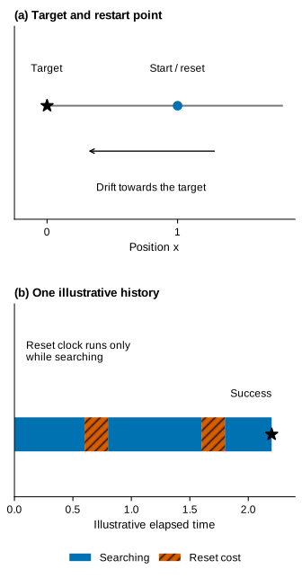
Figure 1. The model separates space from elapsed time. The lower timeline is an explicitly constructed schematic, not a simulated trajectory. Blue intervals represent active searching; hatched intervals represent restart costs. The clock that can interrupt the search runs only during active intervals.

The numerical experiment uses dimensionless units with $x_0=D=1$ . This is not a statement that every physical search has those values. The natural diffusive time scale is $x_0^2/D$ , so a dimensional application would first require its own distance and diffusion estimates. Rescaling the axes can translate units; it cannot establish that Brownian motion is an adequate description of the application.

Almost certain success is not a finite average

Begin with $v=r=0$ . Write $T_0$ for the first time the uninterrupted search reaches zero:

T_0=\inf\{t\geq0:X_t=0\}.

The first-passage density for this driftless model is

\begin{aligned} f_0(t)&=\frac{x_0}{\sqrt{4\pi D t^3}}\\ &\quad\times\exp\!\left(-\frac{x_0^2}{4Dt}\right),\quad t>0. \end{aligned}

One way to understand this expression is to reflect Brownian paths at their first encounter with the target. That symmetry relates the probability of having crossed the target to a Gaussian displacement probability. Differentiating the resulting arrival probability gives the density above. It is a distribution of times, and is very different from the Gaussian distribution of positions at a fixed time.

Its survival probability is

\begin{aligned} S_0(t)&=\Pr(T_0>t)\\ &=\operatorname{erf}\!\left(\frac{x_0}{\sqrt{4Dt}}\right)\\ &\sim\frac{x_0}{\sqrt{\pi D t}}. \end{aligned}

Here survival means that the search remains unfinished, not that anything biological remains alive. Because $S_0(t)$ tends to zero, the probability of eventually reaching the target is one. However, the approach to zero is slow: at long times the unfinished fraction decays only as the inverse square root of time.

For a nonnegative waiting time, the expectation is the area under its survival curve:

\mathbb E[T_0]=\int_0^\infty S_0(t)\,dt=\infty.

The area diverges even though the curve itself approaches zero. Geometrically, the remaining height keeps shrinking, but not quickly enough to make the infinitely long tail have finite area. This is the central distinction between eventual success and average waiting. An expectation is sensitive to how much probability is spread over very large times, not merely to whether an outcome eventually occurs.

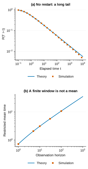
The no-restart survival curve has a slowly decaying tail, while the restricted mean continues increasing as the observation horizon grows. — Figure 2. Uninterrupted searches with zero drift, unit initial distance and unit diffusion. Lines are analytic results; markers summarize 50,000 complete simulations. The lower panel integrates waiting only up to the stated horizon. Its finite values do not imply a finite unrestricted mean.

A finite simulation will nevertheless return a finite arithmetic mean, provided its sampled times are finite. That does not contradict the theory. The simulation contains only finitely many draws from a distribution whose population mean is infinite. Adding another batch may introduce a rare enormous time that changes the sample mean dramatically. Reporting a conventional confidence interval for a finite population mean would answer a question that this model does not possess.

A better finite-horizon question is how much time is spent waiting before a specified deadline. Define the restricted mean

m(\tau)=\mathbb E[\min(T_0,\tau)] =\int_0^\tau S_0(t)\,dt.

Every unfinished search contributes the full observation horizon, rather than disappearing from the calculation. This quantity is bounded by $\tau$ and has a clear operational interpretation. It is still a different objective from eventual completion time: a policy that is best for a short deadline need not minimize the full expected wait.

There is an especially tempting mistake here. If a study stops after a fixed time and averages only the searches that finished, the slowest searches are systematically removed. The resulting number can look reassuring precisely because the troublesome observations are missing. Recording the unfinished fraction alongside the restricted mean keeps the deadline visible instead of disguising it as a successful-completion sample.

How a new attempt changes the calculation

Let $R$ be the exponential restart time during an attempt. Its survival probability is

\Pr(R>t)=e^{-rt},\qquad r>0.

This clock is independent of the search. It does not detect that a run is unpromising, and it does not become impatient with age. At every moment of active searching, it has the same instantaneous restart rate. Some nearly successful attempts will therefore be interrupted. The policy can still help on average if avoiding very long unsuccessful excursions compensates for those lost opportunities.

Denote the total completion time, including all restart costs, by $T_{r,c}$ . The first attempt gives a renewal identity:

T_{r,c}=\min(T_0,R) +\mathbf 1_{\{R\leq T_0\}}\bigl(c+T'_{r,c}\bigr).

The prime denotes an independent copy with the same distribution. If success occurs first, there is no remaining term. If restarting occurs first, we have spent the clock time, pay $c$ , and face the same complete problem again. This renewal viewpoint is the useful general framework developed by Pal and Reuveni; it does not require drawing every intermediate spatial position. Pal and Reuveni, 2017.

Let $p_r=\Pr(T_0<R)$ be the probability of success in one attempt. Taking expectations and solving for the total mean gives

\mathbb E[T_{r,c}] =\frac{\mathbb E[\min(T_0,R)]+c(1-p_r)}{p_r}.

The numerator is the mean time spent on one attempt and its possible reset cost. The denominator accounts for repeated attempts before success. The expected number of attempts is not one: each failure sends the process back to the same starting distribution. This is why the cost cannot simply be added once to the mean of a zero-cost search.

Independence allows the mean active duration of an attempt to be written as

\begin{aligned} &\mathbb E[\min(T_0,R)]\\ &\qquad=\int_0^\infty S_0(t)e^{-rt}\,dt\\ &\qquad=\frac{1-p_r}{r}. \end{aligned}

The last equality follows by integrating the first-passage density against the exponential factor. Meanwhile, conditioning on the time the search would have taken without interruption gives

p_r=\mathbb E[e^{-rT_0}].

That is the Laplace transform of the first-passage distribution, evaluated at the restart rate. It appears here for a physical reason: a hypothetical completion at time $t$ survives the independent restart clock with probability $e^{-rt}$ . Longer prospective attempts are less likely to escape interruption.

For the drift-diffusion model, the transform can also be obtained from a backward equation. If $u(x)$ denotes the chance of reaching the target before the restart clock when starting at $x$ , then

\begin{aligned} Du''(x)-vu'(x)-ru(x)&=0,\\ u(0)=1,\qquad u(\infty)&=0. \end{aligned}

The bounded exponential solution yields

p_r=\exp\!\left[\frac{x_0}{2D} \left(v-\sqrt{v^2+4Dr}\right)\right].

Substitution gives the central prediction for our experiment:

\mathbb E[T_{r,c}] =\frac{1-p_r}{p_r}\left(\frac1r+c\right).

The formula exposes two competing effects of increasing the restart rate. Individual attempts become shorter, but the chance that any one attempt succeeds also decreases. A faster interruption clock is not a faster search mechanism. It is a different rule for allocating time among independent attempts.

What the simulations actually compare

We test drifts $v=0,1,4$ and restart rates $r=0,0.1,0.5,1,2.5,5,10$ . Each of the 21 parameter combinations has 50,000 independent complete searches, giving 1,050,000 searches in total. All long waits are retained. The experiment does not stop a run at a plotting deadline or discard it for taking too long.

Instead of approximating Brownian paths on a time grid, the simulation samples an uninterrupted first-passage time from its exact distribution. Without drift this is a Lévy–Smirnov distribution; with positive drift it is an inverse Gaussian distribution. That sampled time competes with an independent exponential clock. The earlier event determines whether the search ends or starts another attempt.

This event-based procedure avoids a specific numerical error: a discretized path can cross an absorbing target between two recorded positions. A coarse integrator could miss that success and add fictitious waiting time. Exact first-passage sampling removes that time-step error within the stipulated model. It does not remove uncertainty about whether the model describes a real application.

The simulation records active searching time and the number of restarts separately. The four costs $c=0,0.1,0.5,1$ are then applied to the same retained histories. This is a paired comparison, not four independent experiments. It is legitimate because the clock pauses during each cost interval and the underlying process starts anew afterwards. Changing the cost does not alter the sequence of active attempts under those assumptions.

Analytic mean predictions were checked against the simulations using their Monte Carlo standard errors, and independently against numerical integration of the uninterrupted survival probability. All finite-mean comparisons were within five estimated standard errors; the largest absolute discrepancy was approximately 2.65. That agreement checks implementation and sampling consistency. It does not convert the hypothetical corridor into an empirically validated search environment.

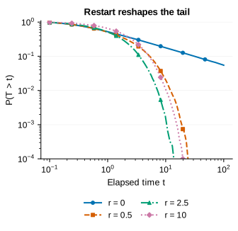
Empirical survival curves compare no restart with restart rates 0.5, 2.5 and 10, showing that excessive interruption loses part of the tail reduction. — Figure 3. Completion-time tails for zero drift and zero cost, with 50,000 searches per rate. Lower curves mean fewer searches remain unfinished at that time. Curves are empirical estimates without confidence bands. Zero observed survivors are omitted on the logarithmic axis; this is not evidence of zero population risk.

At rate 2.5, the observed unfinished proportion at time 5 is 0.04018. At time 10 it is 0.00166. No search in that ensemble remained unfinished at time 30. The last statement describes 50,000 observations, not a hard completion-time guarantee. The model still permits unusually long sequences of unsuccessful attempts.

Notice also what the graph cannot establish: it does not pair a particular restarted run with an uninterrupted run that has the same future. Independent ensembles describe policy distributions. They do not demonstrate that every searcher would personally benefit from restarting. Even a distributional improvement in a chosen statistic is different from a pathwise guarantee.

Why both rare and frequent restarts can be slow

Set $v=c=0$ . The mean simplifies to

\mathbb E[T_{r,0}] =\frac{e^{x_0\sqrt{r/D}}-1}{r}.

For very small $r$ , the clock rarely interrupts an exceptionally long excursion. The mean therefore grows without bound as $r$ approaches zero. For very large $r$ , most attempts are interrupted before the search has time to traverse the initial distance. The many short failures again produce a large total wait.

Between those limits is a balance. Introduce the dimensionless rate variable $z=x_0\sqrt{r/D}$ . Differentiating the mean shows that its positive stationary point satisfies

z_*=2(1-e^{-z_*}), \qquad r_* = \frac{D z_*^2}{x_0^2}.

The nonzero solution is approximately 1.593624. The equation also has the trivial solution zero, but that is not the finite-mean minimum. Returning to $x_0=D=1$ gives the optimum reported earlier. The scaling matters as much as the numerical value: changing the initial distance changes the appropriate rate quadratically, while changing diffusion changes it linearly.

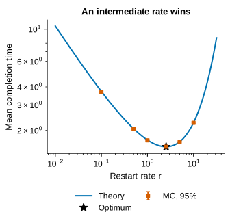
A U-shaped analytic mean-completion-time curve is checked by simulation points and error bars, with an intermediate optimal restart rate marked. — Figure 4. Zero-drift, zero-cost mean completion time. The line is analytic; squares are 50,000-search means with pointwise approximate 95% intervals, calculated as mean plus or minus 1.96 Monte Carlo standard errors. The star marks the analytic optimum, not a fitted minimum of the noisy points. Some error bars are smaller than their markers.

There is no reason to operate at a numerically exact optimum in an application whose parameters are uncertain. A broad low region can be more informative than many reported decimal places. Here the tested rate 2.5 is close enough to the analytic optimum that their theoretical means differ very little. The experiment verifies the shape and scale of the tradeoff, not the operational importance of the sixth decimal place.

The optimization also has a defined policy class. We vary constant-rate, position-independent Poisson restarts. We do not compare all deterministic schedules, position-aware rules, or adaptive strategies. Calling this the optimal search policy without that qualification would turn a precise result into a much stronger unsupported claim.

The average search and the unfortunate search

An average is one way to summarize a distribution, not a universal definition of performance. The median is the time by which half the searches finish. The 90th percentile leaves one tenth unfinished; the 99th percentile leaves one hundredth unfinished. A deadline-sensitive application may care about one of those tail probabilities more than about the mean.

The zero-drift, zero-cost ensembles give the following empirical summaries. Each row represents 50,000 complete searches; “infinite” in the first row refers to the theoretical mean rather than a simulated arithmetic value.

Restart rate	Mean	Median	90th percentile	99th percentile
0	Infinite	1.113	30.936	2611.378
0.1	3.678	1.094	10.183	32.623
0.5	2.045	1.032	5.308	12.130
1	1.709	1.016	4.204	8.751
2.5	1.545	1.047	3.537	7.247
5	1.672	1.171	3.779	7.581
10	2.259	1.573	5.153	10.214

The striking change is in the tail, not in the typical quick completion. Without restarting, the observed median is about 1.113, while the observed 99th percentile is over 2600. At rate 2.5 the median remains near one, but the 99th percentile falls to approximately 7.247. Restarting reorganizes the long waits much more dramatically than it accelerates the already quick searches.

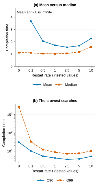
Two panels contrast sample means and medians with upper completion-time quantiles across seven restart rates; the no-restart mean is explicitly infinite. — Figure 5. Different summaries emphasize different parts of the same zero-drift, zero-cost ensembles. Horizontal positions index the seven tested rates rather than a continuous linear rate scale. Lines only connect those summaries. The lower panel uses logarithmic time; quantiles are empirical estimates, not certified deadlines.

The smallest observed median occurs at rate 1 among the tested values, whereas the smallest observed mean occurs at rate 2.5. This is a descriptive comparison of this grid and sample. We have not optimized the population median continuously, nor attached uncertainty intervals to every quantile. Small differences between nearby medians should not be promoted into a precisely located universal optimum.

Tail estimation needs particular care. In 50,000 observations, a 99th percentile is informed by roughly 500 observations beyond it. In a slowly decaying tail, modest uncertainty in the probability level can correspond to a large uncertainty in time. A displayed quantile with three decimals is a rounded computation, not three decimals of established physical precision.

The correct question therefore comes before the optimizer. Are we trying to reduce average resource use, ensure that most searches finish quickly, or reduce the probability of violating a deadline? These objectives can agree over much of the parameter space and still disagree near their optima. Reporting several relevant summaries makes that disagreement visible instead of concealing it behind a single score.

Starting over is not free

Consider a reset that requires restoring a device, rebuilding a state, or waiting for another attempt to become possible. Our $c$ represents elapsed time, not monetary expenditure or energy. Converting it into either of those would require additional assumptions about resource consumption.

For any retained history, the accounting identity is

T_{r,c}=T_{\mathrm{active}}+cN_{\mathrm{reset}}.

The number of failed attempts before the first success has a geometric distribution. Consequently,

\mathbb E[N_{\mathrm{reset}}]=\frac{1-p_r}{p_r}.

A strategy that interrupts frequently pays the cost frequently. At zero drift and rate 2.5, the mean observed restart count is 3.864080, compared with the analytic value 3.860488. At rate 10, the observed count rises to 22.588180. A seemingly modest cost attached to each interruption can dominate the total completion time.

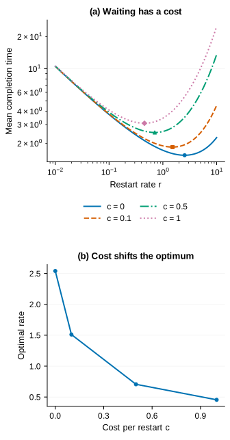
Four analytic completion-time curves show increasing restart costs, with the preferred restart rate decreasing as cost grows. — Figure 6. Analytic zero-drift mean times at costs 0, 0.1, 0.5 and 1. Markers on the upper curves denote optimized rates. The lower panel connects the four computed optima as a visual guide; it does not represent an additional simulation or a fitted universal law.

The optimized zero-drift comparison is:

Cost per restart	Optimal rate	Minimum mean time
0	2.539638	1.544139
0.1	1.510998	1.842512
0.5	0.705919	2.523783
1	0.454764	3.079879

As the cost increases, it becomes sensible to give each attempt more time. The optimizer does not abandon restarting in these driftless examples, because the uninterrupted mean remains infinite while a positive finite rate gives a finite mean. That conclusion is specific to this baseline and the mean objective. It does not mean any finite restart cost is harmless, or that a rate tuned for free resets remains sensible after costs are introduced.

The reset convention itself must be stated. Charging before every attempt, including the first, would add an initial preparation cost. Allowing the environment to evolve during a reset might make the next attempt different from the previous one. Letting the restart clock continue during setup could introduce further interruptions. The refractory-period literature discusses such distinctions; our calculation uses the simpler convention of a fixed pause after each failed attempt. Evans, Majumdar and Schehr, 2020.

Where the waiting time goes

Figure 7 unpacks the cost rather than adding another overall performance score. At $c=0.5$ , it separates the sample mean of active searching from half the sample mean restart count. The two pieces sum exactly because they come from the same completed histories.

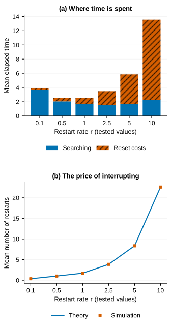
Stacked mean times separate active searching from reset overhead at cost 0.5, with a second panel checking the mean restart counts against theory. — Figure 7. Zero-drift time budgets at cost 0.5, using 50,000 searches per rate. Hatched segments are cost times restart count, not uncertainty bands. The lower panel compares empirical counts with the geometric-distribution prediction. Bar heights use paired histories, so the decomposition is exact at sample level.

This distinction is useful when diagnosing a poor policy. A large total might come from long active excursions, from excessive repeated setup, or from both. Those diagnoses point towards different changes. Increasing the restart rate can shorten active searching over part of the range while simultaneously increasing overhead. Looking only at the total would hide that tradeoff.

The paired construction also avoids an unnecessary source of noise. Comparing costs using different random histories would mix a deterministic accounting change with differences between simulated searches. Holding the active histories fixed isolates the cost effect. However, the same construction would become invalid if cost changed the search dynamics. Pairing is justified by a model assumption, not by an automatic preference for cleaner-looking curves.

When continuing is the better decision

Now add directional progress. For $v>0$ , an uninterrupted drift-diffusion search has

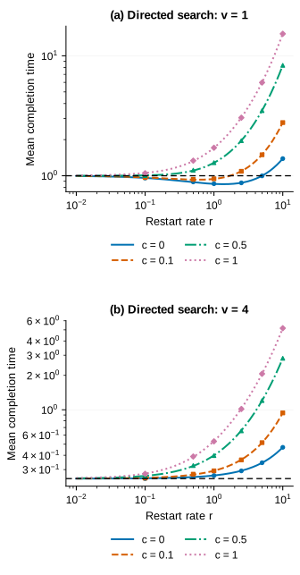
\mathbb E[T_0]=\frac{x_0}{v}, \qquad \operatorname{Var}(T_0)=\frac{2Dx_0}{v^3}.

The infinite-mean baseline has disappeared. Restarting must now beat a finite alternative, rather than merely regularize a divergent expectation. At $v=1$ , the uninterrupted mean is 1. With zero reset cost, optimizing the constant rate gives approximately 1.372008 and a mean of 0.850953. Some restart remains useful, but the improvement is much smaller than the dramatic driftless comparison.

At $v=4$ , the uninterrupted mean is 0.25. The optimization chooses no restart for all four examined costs. For example, at rate 2.5 with zero cost, the analytic mean is approximately 0.292961, already worse than continuing. With cost 1, that mean becomes approximately 1.025365. A mechanism that rescued wandering searches now interrupts comparatively reliable progress.

Separate panels for drift one and drift four compare restart policies against finite no-restart means, exposing cases where restart increases waiting. — Figure 8. Directed-search controls with unit distance and diffusion. Lines are analytic means and markers are 50,000-search means; colours, line styles and markers identify the four costs. Black dashed lines mark the exact no-restart means, 1 and 0.25. Costs reuse the same active histories within each rate.

A local calculation explains the transition. Suppose an uninterrupted completion time has finite mean $m$ and finite second moment. Expanding its Laplace transform around zero gives the initial response of the restarted mean:

\left.\frac{d\mathbb E[T_{r,c}]}{dr}\right|_{r=0} =\frac{m^2-\operatorname{Var}(T_0)}{2}+cm.

Writing the coefficient of variation as $\mathrm{CV}=\sqrt{\operatorname{Var}(T_0)}/m$ , a small amount of restarting improves the mean when

\mathrm{CV}^2>1+\frac{2c}{m}.

Large variability can make restarting useful, but setup cost raises the required variability. For our drift-diffusion model, $\mathrm{CV}^2=2D/(vx_0)$ . Thus $v=1$ and $v=4$ sit on different sides of the zero-cost local condition. At $v=1,c=0.5$ , the first derivative is zero; that alone does not decide the global optimum, so the full mean curve must still be examined.

This expansion does not apply to the zero-drift infinite-mean case. It also provides a local statement about introducing a small restart rate, not a proof that every larger rate helps. Keeping those qualifications is part of understanding the calculation, rather than an administrative restriction attached to it.

What to measure before recommending a restart

The opening question sounded like a choice about persistence. The model turns it into a choice about information and time allocation. Before transferring its conclusion to another setting, we need to know whether the assumptions that create a renewal are plausible.

First, does restarting actually restore the same starting distribution? A solver that retains learned information, a device whose battery drains, or an environment that changes during setup does not begin an independent copy of the original attempt. Such memory may improve or worsen the value of restarting. It must enter the model explicitly rather than being silently discarded.

Second, is elapsed time the only observation available? Our clock ignores current position and evidence of progress. If a searcher knows it is close to the target, a state-dependent policy might avoid an especially damaging interruption. If only completion times are observed, estimating the residual waiting distribution becomes more relevant. The best policy depends on the information available when the decision is made.

Third, what counts as success? We have assumed a fixed, perfectly absorbing target. Detection failures, moving targets and multiple possible outcomes change the completion law. A reset that returns the searcher but not the target can fail to renew the problem. The visual metaphor of returning to the start is not enough; the relevant statistical state has to return as well.

Fourth, which cost is binding? Time spent resetting is only one possibility. Energy, wear, communication limits and the risk of losing a recoverable state may all matter. A policy minimizing expected elapsed time need not minimize any of those. There is no contradiction if a slower time policy is preferred under a different objective.

Finally, what evidence would distinguish useful restarts from selection effects? Keep unsuccessful and unfinished attempts in the records. State observation horizons. Compare policies on compatible starting conditions. Separate uncertainty in the observed sample from uncertainty in the model itself. A very precise simulation of an inappropriate renewal model can still recommend the wrong action.

Conclusion

Starting over can make a random search finish sooner because accumulated motion is not necessarily accumulated progress. In the driftless model, restarting prevents rare wandering excursions from dominating the mean. An intermediate rate balances that benefit against the chance of interrupting an attempt that might soon succeed.

The same calculation explains its limitations. Excessive interruption produces many failures. Setup time makes those failures expensive. Directional progress reduces the value of abandoning the current attempt. And an optimizer for the mean does not automatically answer a question about a deadline or the slowest searches.

The next useful question is therefore not simply “should we try again?” It is: what distribution will a new attempt draw from, what must be paid to obtain it, and which waiting times are we trying to improve? Those questions make restarting a testable modeling decision rather than a slogan about persistence.

References

Evans, M. R., and Majumdar, S. N. (2011). Diffusion with Stochastic Resetting. Physical Review Letters, 106, 160601. Classical diffusive first-passage benchmark.
Pal, A., and Reuveni, S. (2017). First Passage under Restart. Physical Review Letters, 118, 030603. General renewal formulation for completion under restart.
Evans, M. R., Majumdar, S. N., and Schehr, G. (2020). Stochastic Resetting and Applications. Journal of Physics A: Mathematical and Theoretical, 53, 193001. Broader context, including restart conventions and refractory periods.