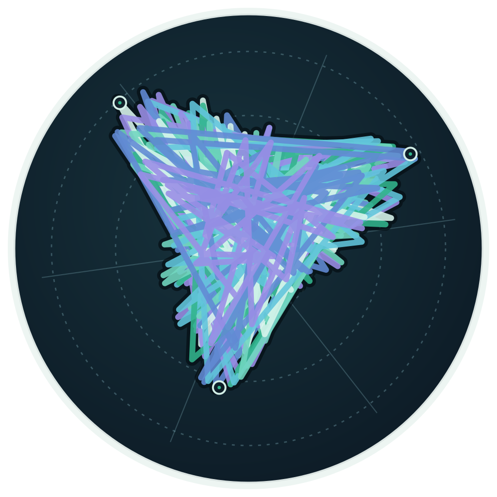
When Solar Power Changes Fast: Why Better Intervals Are Still Not Reliable Enough

Imagine a solar operator looking at a forecast just as a cloud bank crosses the site. The central prediction changes, and a shaded band offers reassurance: this is a 90% prediction interval. The operator is not expecting perfect foresight. They want to know how much confidence to place in the range when generation changes quickly and some of the measurements used by the model are unavailable.

This is a hypothetical operating scene, not a deployment evaluated in our study. It nevertheless exposes the question behind the research. Does the number attached to an uncertainty band describe the moments when it is most needed, or mainly the more ordinary moments that dominate the data?

There are two different ways to improve that band. One is to make it perform better than an existing method. The other is to make it sufficiently reliable for a stated purpose. A method can succeed at the first and fail at the second. Our solar forecasting results provide a concrete example: calibration improved all five confirmation stations, while the weakest evaluated groups remained a long way from the intended coverage.

This article explains our accepted ADMA 2026 short paper through that distinction. It is an empirical study of public energy data, not a new theorem guaranteeing conditional coverage. The project overview records the research and author information; the student research studio places it within the mentoring programme.

What the solar experiment found

We evaluated five stations across four chronological folds and two forecast horizons, giving 40 station–fold–horizon combinations. The leading calibration candidate, Descriptor CQR, reduced mean station worst-group undercoverage by 0.110 at 15 minutes and 0.080 at 60 minutes. Those are absolute changes in coverage shortfall, equivalent to 11.0 and 8.0 percentage points, not relative percentage improvements.

The remaining worst shortfalls were 0.430 and 0.363 below a nominal coverage target of 0.90. The corresponding observed group coverages were only 0.470 and 0.537. These are the hardest eligible groups, not overall averages. Neither number should be presented as evidence that a nominal 90% interval achieved 90% in practice.

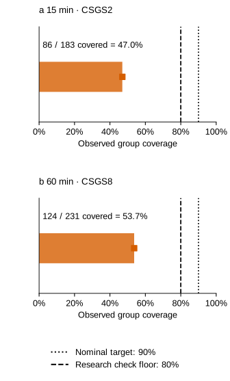
Two panels compare Descriptor CQR worst-group coverage of 47.0 and 53.7 percent with the 80 percent research floor and 90 percent nominal target. — Figure 1. Descriptor CQR still falls below the reliability check. At 15 minutes, the CSGS2 weather-outage ramp group in the first 2020 test quarter covers 86 of 183 targets; at 60 minutes, the corresponding CSGS8 group covers 124 of 231. The dotted 90% line is the nominal target. The dashed 80% line is this study's deliberately permissive checking floor, not an industry standard. Counts are observations within selected groups, not independent station replications.

The contrast is already visible without knowing how the models work. Moving an interval method in the right direction does not establish that it has arrived. We therefore need to understand both the meaning of coverage and the sequence of choices that determines which observations enter its denominator.

What does the 90% actually describe?

At forecast time, an interval supplies a lower endpoint and an upper endpoint. Once the future power measurement arrives, we can ask whether that measurement lies between them. Coverage is the fraction of evaluated targets contained in their respective intervals. It describes a repeated forecasting procedure, not a claim that every particular interval has been assigned a separately verified probability.

Even an accurate overall coverage estimate leaves a second question unanswered: coverage conditional on what? Suppose, purely as an arithmetic illustration, that 90% of forecasts concern ordinary conditions and achieve 95% coverage, while the other 10% concern difficult events and achieve 45%. The pooled coverage is exactly 90%. A reassuring overall number can coexist with poor performance in a consequential minority. This illustration is not an additional experimental result.

Our study separates three counts within each evaluated group. Let the number of attempted forecasts be $A_g$ , the number of issued intervals be $I_g$ , and the number of covered targets be $K_g$ . Then

\widehat C_g=\frac{K_g}{I_g},\qquad \widehat C_g^{\mathrm{service}}=\frac{K_g}{A_g}.

The first is issued-interval coverage. The second is service coverage: an attempted forecast that produces no interval counts as uncovered. Neither definition is interchangeable with the other. A service that declines its hardest cases may look impressive when evaluated only on the forecasts it manages to issue.

For the primary baseline and three main candidates in this experiment, every attempted interval was issued. Their two coverage measures therefore coincide. This is a property of these saved evaluations, not a promise about future availability. Width and interval score are still defined only for issued intervals; assigning an artificial zero width to an unavailable prediction would reward failure to produce an answer.

There is another population boundary before either denominator. The study requires observed current power and an observed future target for its main evaluation and ramp labels. An origin excluded before forecasting is not secretly included in the service denominator. We return to this distinction when examining natural missingness, because it limits what even 100% prediction availability can mean.

Why inspect stations and events separately?

The data come from the public Chinese State Grid competition dataset documented by Chen and Xu: measurements collected every 15 minutes during 2019–2020. We use its solar-site files, not a simulated solar plant. The original dataset is described in the data paper.

CSGS1 was reserved for development. Seven other station files were screened using data-integrity rules before comparing method outcomes. Five remained: CSGS2, CSGS5, CSGS6, CSGS7 and CSGS8, with nominal capacities of 130, 110, 35, 30 and 30 MW. CSGS3 lacked a required temperature column. CSGS4 had 25.720% missing daylight targets, above the prespecified 20% exclusion threshold. Neither was removed because a forecasting method performed badly there.

This separation protects the interpretation of external confirmation. A development station can help formulate a promising approach; it should not then be counted as fresh evidence that the approach generalizes. Equally, data screening should establish whether a comparison can be conducted, not select the sites that produce a preferred conclusion.

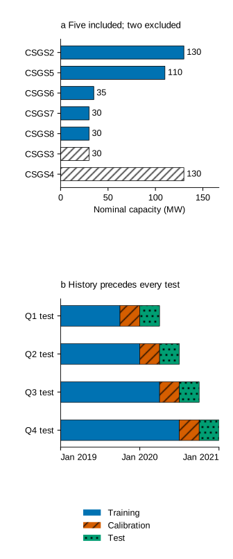
Station capacities for five included and two excluded solar sites appear above four expanding chronological training, calibration and test windows. — Figure 2. The five confirmation stations span nominal capacities from 30 to 130 MW. Hatched bars identify the excluded CSGS3 and CSGS4 files; CSGS1 is development-only and is not a confirmation bar. Each training period precedes a calibration quarter and a disjoint 2020 test quarter. Origins whose future targets cross a split boundary are purged. The timeline shows chronological blocks, not independent repetitions or station geography.

Each retained site is evaluated at 15 and 60 minutes. The four test quarters run through 2020. The first training window ends in September 2019, followed by calibration in October–December and testing in January–March 2020. Later folds expand the history and move calibration and testing forward by one quarter. The last training window ends in June 2020, followed by third-quarter calibration and fourth-quarter testing.

Why not shuffle the timestamps? Because a forecasting procedure should not learn from the period it is supposed to predict. More subtly, a training origin just before a boundary can have a target after that boundary. Target-time purging removes these crossings. Merely sorting the input timestamps would not, by itself, prevent the future response from leaking across a split.

The four test quarters are disjoint, but the folds reuse earlier history. They are not four independent experiments at each station. Nor are the many timestamps independent samples of geographical generalization. The statistical replication unit is the station. Forty evaluation combinations describe the design; five stations describe the available external replication.

For ordinary averages, eligible fold–sensor–event groups are first averaged equally within each station, and station averages then receive equal weight. This answers a station-first question. Pooling all rows instead would give more influence to sites or groups with more observations. Both can be meaningful estimands, but they are not the same estimand with different formatting.

A ramp is an evaluation definition, not advance knowledge

Write power at station $s$ and time $t$ as $y_{s,t}$ , and its nominal capacity as $C_s$ . With horizons measured in 15-minute steps, the event label is

\begin{aligned} r_{s,t,h}&=\mathbf 1\!\left\{ \frac{|y_{s,t+h}-y_{s,t}|}{C_s}\geq\tau_h \right\},\\ \tau_1&=0.10,\quad\tau_4=0.20. \end{aligned}

A ramp therefore means a sufficiently large absolute change relative to station capacity. Both upward and downward changes qualify. Normalization makes a given fractional change comparable across differently sized sites without pretending that their physical environments are identical.

The two thresholds are not equivalent ramp rates: a 10% change over 15 minutes and a 20% change over 60 minutes describe different event selections. They are retained research definitions, not universal physical tipping points, dispatch limits or official operational standards. Changing them changes the question being asked of the predictions.

Most importantly, the realized label uses future power. It is available for evaluation after the outcome arrives, but not when an interval must be issued. A deployable method may estimate ramp risk using current information. It cannot use the true future ramp label and still be described as operating with forecast-time information.

A separate recent study of national-scale solar ramps motivates treating rapid changes as a distinct forecasting problem, but it does not validate our five-site results or establish their geographical representativeness. Its scale and models differ from ours. See Lanzilao and Meyer for that complementary perspective.

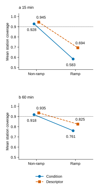
Condition and Descriptor CQR have higher mean station coverage in non-ramp groups than in ramp groups at both 15 and 60 minutes. — Figure 3. Mean station coverage separates ordinary changes from ramps. At 15 minutes, Condition and Descriptor coverage is 0.928 and 0.945 for non-ramps, versus 0.583 and 0.694 for ramps. At 60 minutes the corresponding values are 0.918 and 0.935, versus 0.761 and 0.825. Each method and horizon has 100 eligible groups per stratum: five stations, four folds and five sensor conditions. Groups are averaged within station, then across five stations; markers are point estimates, not confidence intervals. The dotted line marks nominal 0.90 coverage.

The figure explains why a single average is insufficient. Calibration improves both strata, but a substantial ramp deficit remains. It also explains why the worst group can be much worse than the mean ramp group. The latter averages across sites, seasons and sensor conditions; the former deliberately asks where that averaging is least reassuring.

How the calibration changes the interval

The principal comparison holds the underlying forecaster fixed. Condition CQR, Descriptor CQR, Risk-Mondrian, Rolling CQR and the future-label diagnostic share a degradation-augmented Extra-Trees model within each station–fold–horizon run. Changes among them therefore concern calibration on a shared forecasting base, not a contest in which every method receives a different predictor.

The base interval is initialized from empirical quantiles of individual tree point predictions. These are not quantiles of all responses stored in forest leaves. The distinction matters because agreement among fitted trees is not automatically a well-calibrated account of future outcome uncertainty. Calibration uses observed errors to adjust the initial band.

Conformalized quantile regression, introduced by Romano, Patterson and Candès, provides the general starting point. The expansion-only score used here is

a_i=\max\{\widehat q_\ell(x_i)-y_i, y_i-\widehat q_u(x_i),0\}.

If the observation is inside the base interval, this score is zero. If it lies below the lower endpoint or above the upper endpoint, the score records the expansion needed to include it. The explicit zero makes this version expansion-only: calibration does not use a negative correction to shrink an already generous base interval.

For a nonnegative correction $q(x)$ , the final endpoints are

\begin{aligned} L(x)&=\max\{0,\widehat q_\ell(x)-q(x)\},\\ U(x)&=\min\{C_s,\widehat q_u(x)+q(x)\}. \end{aligned}

Clipping retains the model’s physical output range. It does not turn an empirically estimated correction into a universal reliability guarantee. How we choose the correction, what information it uses, and how representative the calibration period is all remain important.

Four ways to decide how much expansion is needed

Condition CQR groups calibration scores by the known sensor condition. A weather-input outage need not receive the same correction as a clean-input forecast. This baseline recognizes missing information, but a single condition-level correction still averages over different event risks within that condition.

Risk-Mondrian adds four forecast-time risk strata. A separately trained Extra-Trees classifier estimates ramp risk using training data and available descriptors. Calibration scores are grouped by condition and risk bin. Small groups are stabilized by blending their correction with the condition-level correction, using weight $n/(n+100)$ for a bin containing $n$ calibration observations. An empty bin falls back to the condition correction. This shares information rather than treating a sparse group estimate as equally trustworthy.

Descriptor CQR models the score directly. A LightGBM quantile model uses 15 descriptors: estimated risk, capacity-normalized base width and median, three family-level missing fractions, observed-context fraction, hour sine and cosine, transition risk, and five condition indicators. It is a score model with chronological residual calibration, not nearest-neighbour calibration. The model attempts to adapt expansion to a description of the forecast situation rather than a distance-based set of neighbouring examples.

The earliest 60% of unique calibration times fit that score model. The latest 40% provide residuals for a separate correction. If the estimated score quantile is $\widehat q(x)$ , the final correction has the form

\begin{aligned} q(x)&=\max\{\widehat q(x)+\kappa,0\},\\ \kappa&=\max\{0,Q_{1-\alpha}^{\mathrm{residual}}\}. \end{aligned}

Here $\alpha=0.10$ . The residual quantile uses the finite-sample rank $\lceil(n+1)(1-\alpha)\rceil$ , bounded to the available range from 1 to $n$ . Unique timestamps define the split so that multiple condition copies of one time do not straddle its two parts. Separating model fitting from residual correction avoids evaluating calibration on the same errors used to fit the score relationship.

Rolling CQR instead uses the latest 500 released scores for each condition, requiring at least 100. The word released matters. A 60-minute forecasting error does not become observable immediately after the forecast is issued; its target must first arrive. Updating a rolling calibrator prematurely would feed it information from the future.

These mechanisms offer different responses to heterogeneity and time variation. None removes the need to evaluate difficult groups. Work on sequential predictive conformal inference studies residual dependence, while adaptive conformal prediction examines adaptation over time. Their theoretical results depend on their stated methods and assumptions; they are not inherited automatically by this empirical pipeline.

What was actually removed from the inputs?

The study evaluates five conditions: clean inputs, irradiance-feature removal, weather-feature removal, recent-power-feature removal, and their combined removal. The separate feature families contain 9, 9 and 13 features; the combined condition removes their union of 31. Targets remain observed and are not interpolated.

This is a controlled way to ask how forecasts respond to missing information at the forecasting origin. It is not a full model of instrument ageing, outage duration, communication recovery, noise bursts or measurement drift. The forecaster is trained with degraded examples, so these tests also do not represent an entirely unforeseen type of failure. Their value is comparability: methods face the same recorded targets under specified information restrictions.

Improvement is a comparison; reliability is a requirement

For each eligible group, define undercoverage relative to the 90% target. For each station and horizon, take the largest such shortfall:

\begin{aligned} u_g&=\max\{0,0.90-\widehat C_g\},\\ W_{s,h}^{(m)}&=\max_{g\in\mathcal G_{s,h}}u_g. \end{aligned}

Groups require at least 80 issued intervals. This removes very small cells, but 80 is not a theorem about precision. Successive forecasts can be dependent, and the maximum searches across multiple cells. A selected worst-group estimate should not be read as a noise-free population parameter.

Our deliberately permissive absolute check is

W_{s,h}^{(m)}\leq0.10\quad\text{at every station}.

Because the target is 0.90, this allows eligible group coverage as low as 0.80. It is a research checking floor, not a statement that 80% is satisfactory for grid operations. It is also not a significance test or an industry standard. Even clearing this floor would leave operational validation to be done.

The comparative check asks a different set of questions: is mean station improvement at least 0.05, do at least 60% of stations improve, is the saved station-bootstrap upper bound for candidate-minus-baseline worst shortfall below zero, and is the clean-condition proper-score ratio no more than 1.10? The mean paired improvement is

\overline\Delta_h=\frac{1}{5}\sum_s \left(W_{s,h}^{\mathrm{Condition}}-W_{s,h}^{\mathrm{candidate}}\right).

Positive values favour the candidate. The pairing keeps station identity intact. A large improvement on one station should not be treated as evidence that a different station benefited; each comparison starts with its own baseline.

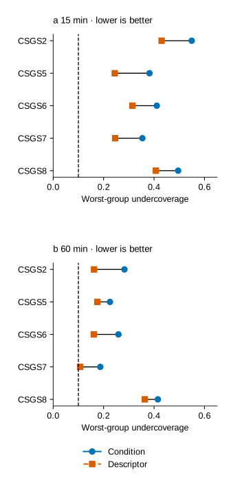
Paired station points show that Descriptor CQR reduces worst-group undercoverage at every station, while every result remains above the 0.10 tolerance. — Figure 4. Five paired station comparisons at each horizon. Blue circles are Condition CQR and orange squares are Descriptor CQR; each connector joins the same station, not a confidence interval. Every pair improves, but every Descriptor endpoint remains above the dashed 0.10 shortfall tolerance. The worst group can differ between methods, so connectors compare station endpoints rather than the same selected timestamp group.

Descriptor CQR meets the comparative criteria at both horizons. Risk-Mondrian does so only at 15 minutes; its 60-minute mean improvement of 0.040 is below the required 0.05. Rolling CQR meets neither comparative check. No deployable candidate meets the absolute criterion.

Horizon (min)	Candidate	Mean improvement	Comparative criterion	Absolute criterion
15	Descriptor CQR	0.110	Met	Not met
15	Risk-Mondrian	0.079	Met	Not met
15	Rolling CQR	-0.002	Not met	Not met
60	Descriptor CQR	0.080	Met	Not met
60	Risk-Mondrian	0.040	Not met	Not met
60	Rolling CQR	0.022	Not met	Not met

There is useful negative evidence here. A more recent calibration window is not automatically a better description of the next difficult event. Rolling’s 15-minute mean change is slightly adverse, rather than merely an unreported tie. Its 60-minute improvement is positive but insufficient. These are outcomes of the specified procedure, not evidence that every possible rolling method must fail.

The five-site design also limits the strength of uncertainty statements. Station-level bootstrap calculations summarize variation among the observed stations; they do not create additional sites. Showing the individual pairs remains important even when a summary interval supports a favourable average comparison. The common data source and limited number of stations prevent a broad geographical or climatic reliability claim.

Wider intervals are not a free improvement

An interval spanning every plausible power value would often cover the target, but offer little discrimination. Coverage alone therefore rewards a trivial response to uncertainty: make every band wider. The study reports width alongside a proper interval score that also penalizes misses.

For $\alpha=0.10$ , the score is

\begin{aligned} S_\alpha(L,U;y)={}&(U-L)\\ &+\frac{2}{\alpha}(L-y)\mathbf 1\{y<L\}\\ &+\frac{2}{\alpha}(y-U)\mathbf 1\{y>U\}. \end{aligned}

The first term charges for width. The other terms charge for the distance of a miss below or above the interval. A distant miss is worse than one just outside the endpoint. Dividing both width and score by station capacity makes the reporting scale comparable across the differently sized stations. Lower score is better.

The coefficient $2/\alpha$ is 20 here. As a hypothetical example, an interval of normalized width 0.20 with a target 0.05 above its upper endpoint receives a score of 1.20. Widening the upper endpoint enough to include that target increases the width charge but removes a larger miss penalty for that observation. Across many cases, however, widening also charges observations that were already covered. The aggregate trade-off must be measured.

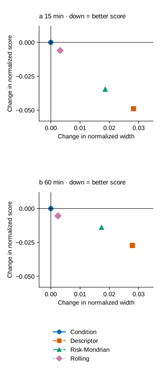
Scatter panels show wider intervals but lower aggregate proper interval scores for the three calibration candidates relative to Condition CQR at both horizons. — Figure 5. Width–score trade-offs relative to Condition CQR at 15 and 60 minutes, with equal weighting of eligible groups within each of five stations and then across stations. Rightward means wider intervals; downward means a better normalized proper interval score. Descriptor width rises by 0.028 at both horizons while score changes by -0.049 and -0.027. All four primary methods issue every attempted interval in these evaluations. Points are saved aggregate estimates; no uncertainty bands are implied.

Descriptor’s mean normalized width increases by 0.028 at both horizons. Its normalized proper score decreases by 0.049 and 0.027. This is evidence that wider bands can improve the combined coverage–sharpness assessment, not merely inflate coverage without any other benefit.

But that conclusion should not erase the groups where the trade-off worsens. At 15 minutes, non-ramp coverage improves by 0.017 and width increases by 0.012, while normalized score becomes worse by 0.001. For ramps, the changes are +0.110 coverage, +0.045 width and -0.099 score. The larger ramp benefit explains why the aggregate can improve while ordinary cases pay a small efficiency cost.

At 60 minutes, the non-ramp changes are +0.017 coverage, +0.015 width and -0.004 score; the ramp changes are +0.065, +0.040 and -0.051. These are averages of the relevant groups, not the worst-group endpoints shown earlier. A reader should not subtract a stratum-average score change from a station maximum and interpret the result as a new performance measure.

Prior photovoltaic conformal forecasting research supplies useful context for interval calibration. Our result adds a narrower warning: improving an aggregate interval score does not, by itself, repair the weakest conditional coverage. Whether an interval is useful in an actual control decision would additionally depend on the decision rule, asymmetric consequences and available responses. None of those dispatch outcomes was measured here.

Why future labels are not a performance ceiling

It is tempting to ask what would happen if the calibrator knew whether a ramp was coming. The study includes a reference that uses realized future ramp labels. This is deliberately unavailable information at forecast time, so the comparison is diagnostic rather than deployable.

One might call this a perfect-information ceiling and divide the remaining gap into an information component and a calibration component. That interpretation is not justified. Knowing the label changes how calibration observations are grouped; it does not guarantee that the estimated correction from those groups will dominate another method. Finite calibration samples, different grouping and a worst-group objective can all complicate the comparison.

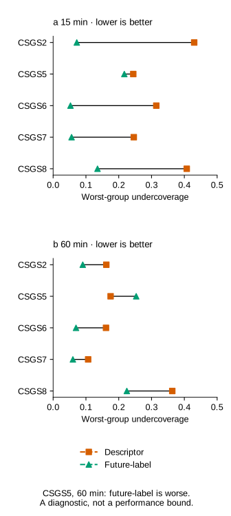
Direct station comparisons of Descriptor CQR and the non-deployable future-label diagnostic highlight CSGS5 at 60 minutes, where the future-label result is worse. — Figure 6. Descriptor CQR versus a reference using realized future ramp labels, paired across five stations at each horizon. The reference is unavailable at forecast time. At CSGS5 and 60 minutes, Descriptor worst-group undercoverage is 0.175, whereas the future-label value is 0.253. The reversed ordering is retained. Connectors are descriptive comparisons, not additive components, causal effects, error bars or a guaranteed performance bound.

CSGS5 at 60 minutes is the decisive counterexample: the future-label reference has worse worst-group undercoverage, 0.253 rather than Descriptor’s 0.175. A method with extra information is not necessarily a better finite-sample procedure for every site and criterion. That observation does not mean future information is intrinsically harmful; it means this particular reference is not an optimum over everything one could do with that information.

The median Descriptor-minus-reference shortfall gap is 0.262 at 15 minutes and 0.072 at 60 minutes. Those summaries may help formulate questions about useful forecast-time descriptors, but they do not identify causal contributions. We did not intervene on atmospheric information while keeping every other mechanism fixed, and no decomposition theorem was established.

This is also why the figure uses paired comparisons rather than stacked bars. A stack would visually suggest that the total shortfall can be partitioned into nonnegative explanatory pieces. Here the sign can reverse. The honest scientific question is whether improved forecast-time risk information can reduce difficult-group error in a new evaluation, not how much of the current error has already been causally assigned to missing knowledge.

Does the conclusion depend on the event threshold?

The saved predictions can be evaluated under alternative ramp definitions without fitting models again. At 15 minutes, the threshold is varied across 7.5%, 10% and 15% of capacity. At 60 minutes, it is varied across 15%, 20% and 25%. The interval predictions themselves remain fixed.

This is a sensitivity analysis of evaluation labels. The training weights, risk classifier labels, calibrators and future-label reference retain their nominal definitions. It would be inaccurate to describe these curves as separately optimized pipelines for each threshold. A new training study at alternative thresholds could behave differently.

No-refit threshold sensitivity shows rising worst undercoverage and shrinking ramp support, with only four evaluable stations at the highest threshold in each horizon. — Figure 7. Worst undercoverage among eligible groups under alternative event labels, using unchanged predictions. Tick labels report ramp-evaluable stations and eligible fold–condition ramp cells, each requiring at least 80 issued intervals. The 15-minute support counts are 100, 100 and 70 cells; the 60-minute counts are 100, 100 and 80. At the highest thresholds, CSGS8 has no eligible ramp cells, leaving four ramp-evaluable stations. Some Condition and Rolling points intentionally coincide. Curves connect evaluated thresholds, not a fitted continuous law.

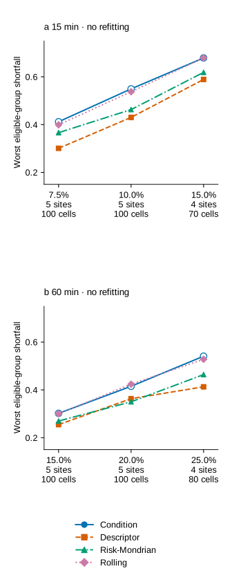
The 15-minute ramp-origin counts fall from 12,928 to 8,269 to 3,946. At 60 minutes they fall from 24,267 to 13,718 to 6,903. These are origin counts, not fivefold copies across sensor conditions. A stricter threshold selects fewer and larger changes, so both event difficulty and sample support change together.

At the highest 15-minute threshold, CSGS2 retains only 10 eligible ramp cells, three other sites retain 20 each, and CSGS8 retains none: 70 in total. At the highest 60-minute threshold, four sites retain 20 each and CSGS8 again retains none: 80 in total. A zero in that support count means no eligible cell; it is not an observed zero error rate.

Descriptor’s worst eligible-group shortfall rises from 0.301 to 0.430 to 0.589 across the 15-minute thresholds. The 60-minute sequence is 0.255, 0.363 and 0.413. These values support concern about harder event definitions, while the changing eligible population prevents a simple claim about an unchanged five-site ramp panel.

The checking tolerance can also be varied without changing any prediction. Shortfall tolerances of 0.05, 0.10 and 0.15 correspond to coverage floors of 85%, 80% and 75%. At the loosest of these, only Descriptor at 60 minutes clears the tolerance at one of five stations; none achieves the all-station requirement. Moving a reporting line does not improve a forecast, and sensitivity analysis should not become a search for the line that makes a disappointing result disappear.

What can the naturally missing data tell us?

Synthetic removal provides controlled comparisons, but naturally missing inputs raise a different question. Do the historical records contain enough relevant cases to evaluate what actually happened when measurements were absent?

First consider the population. At 15 minutes, 110,425 daylight test origins have observed future targets; 382 lack current power and are excluded, leaving 110,043 model-evaluable origins. At 60 minutes the corresponding counts are 110,302, 1,348 and 108,954. These exclusions happen before the forecasts and ramp labels used in this analysis. Consequently, the study does not evaluate complete current-power outages.

Next consider conditional support. Natural missingness selects cases from the primary methods’ clean-condition predictions where a relevant feature family was already missing. Structurally absent optional channels are not treated as a continuous sensor failure. Across five stations, four folds, two horizons, four feature families and two event strata, there are 320 family–ramp cells. Only 24 reach the minimum of 80 observations, all at CSGS5.

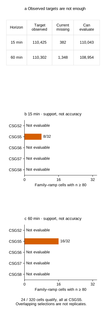
A population table shows excluded missing-current-power origins, while support panels show that only CSGS5 has eligible natural-missingness groups at either horizon. — Figure 8. The scope of natural-missingness evaluation. The top table separates observed future targets, missing-current-power exclusions and model-evaluable origins. The lower panels show eligible family–ramp cells out of 32 per station and horizon: 8 at 15 minutes and 16 at 60 minutes, all at CSGS5. Other sites are marked not evaluable, not error-free. The total 24 of 320 cells includes overlapping feature-family selections; identical timestamp sets are counted once when pooling performance.

The distinction between support and performance is crucial. A bar for eight eligible cells is not an accuracy score. Likewise, two feature-family labels that select exactly the same timestamps are not two replications of the result. The natural-missingness summaries deduplicate identical recent-power and combined selections before pooling their performance.

The selected results contain both benefits and costs. At 15 minutes, the non-ramp subset has 4,189 observations: Descriptor-minus-Condition changes are -0.002 coverage, +0.000 undercoverage, +0.003 normalized width and +0.001 normalized score. At 60 minutes, 3,767 non-ramp observations give +0.020, +0.000, +0.016 and +0.003. Thus wider intervals and higher coverage need not improve score in these selected non-ramp subsets.

For the 614 selected 60-minute ramp observations, the changes are +0.033 coverage, -0.022 undercoverage, +0.028 width and -0.018 score. The coverage gain and undercoverage reduction differ because undercoverage is truncated at zero. Once pooled coverage crosses 0.90, further coverage gains no longer reduce that shortfall. Applying the truncation after pooling also differs from averaging the separately truncated cell shortfalls; the reported natural-missingness comparison uses the pooled quantity.

These results are a post-run descriptive sensitivity, not fresh confirmation across five sites. Research on conformal prediction with missing values helps explain why the pattern of missingness deserves explicit attention. It does not allow this selected CSGS5 subset to stand in for every missingness mechanism or real outage.

The practical next step is therefore partly a measurement problem. Before proposing a more complicated calibrator, one should ask which currently excluded conditions can be observed and evaluated honestly. A future study might need independently recorded outcomes during telemetry loss and a forecast protocol that does not require current power. That is a proposed study design, not evidence already supplied by the present data.

What should be tested next?

Three questions follow naturally. First, can forecast-time descriptors distinguish difficult upcoming events more effectively without using their realized labels? The relevant test would preserve chronological fitting and assess new station-level outcomes, rather than choose descriptors after inspecting the same worst groups.

Second, can interval efficiency be improved where ordinary cases pay for wider bands? A candidate should retain ramp coverage gains while avoiding unnecessary expansion elsewhere. That requires simultaneous reporting of coverage, width and proper score, not a switch of headline metric when one result is inconvenient.

Third, what reliability target corresponds to a real decision? Our study checks two separate horizons, not simultaneous coverage of an entire future trajectory. ConForME illustrates why multi-horizon uncertainty is its own problem. A decision depending on a sequence of power values, storage constraints or asymmetric reserve costs needs an evaluation designed around that decision. Two marginal horizon checks cannot be silently promoted into a guarantee for the whole trajectory.

Each question calls for new evidence. Additional stations would strengthen external replication. Better outage records would expand the evaluable population. A decision-focused experiment would test operational value. None can be replaced by counting more timestamps from the same limited setting as if they were new independent environments.

Conclusion

The most encouraging result is also the reason to resist an overconfident conclusion. Descriptor CQR improves the worst-group endpoint at every confirmation station, and its wider intervals deliver better aggregate proper scores. The gain is real within the evaluated comparison.

Yet the hardest groups still achieve only 0.470 and 0.537 coverage against a nominal target of 0.90. No deployable candidate clears even the deliberately permissive all-station reliability check. The study therefore supports continued work on conditional calibration, not a claim that uncertainty during solar ramps and sensor degradation has been solved.

When the next forecast arrives with a reassuring shaded band, the productive question is not simply whether the method beats a baseline. It is: reliable for which conditions, among which attempted forecasts, at which stations, with what interval width, and for what decision? An uncertainty estimate becomes more useful when those questions become easier to answer.

Research and author record

This article explains When Solar Power Changes Fast: A Multi-Site Audit of Prediction-Interval Reliability under Ramp Events and Sensor Degradation, by Hong U Lo, Zibo Gao, Peng Chi Lam, and Sok Kin Cheng, in the paper’s formal author order. The affiliation is St. Joseph Diocesan College (The Fifth School), Macao SAR, China. Sok Kin Cheng is the corresponding author and student research mentor.

The work was accepted from the ADMA 2026 Research Track as a Short Paper on 3 September 2026. The camera-ready submission was completed on 9 September 2026. The conference is scheduled for 13–15 November 2026 in Hong Kong. Acceptance and submission are the recorded milestones; this page does not claim a completed presentation, published proceedings entry, indexing or an assigned paper DOI.

The numerical discussion follows the submitted eight-page camera-ready paper and its public research version. Figures here are newly drawn from its saved results, not newly trained models. See the project page for a concise overview and the mentoring record for the educational context.

References

Chen, Y., and Xu, J. (2022). Solar and wind power data from the Chinese State Grid Renewable Energy Generation Forecasting Competition. Scientific Data, 9, 577.
Lanzilao, L., and Meyer, A. (2026). Characterization and forecasting of national-scale solar power ramp events. arXiv preprint.
Galvão Lopes, A., Goubault, E., Putot, S., and Pautet, L. (2024). ConForME: Multi-horizon conditional conformal time series forecasting. PMLR, 230, 345–365.
Renkema, Y., Visser, L., and AlSkaif, T. (2024). Enhancing the reliability of probabilistic PV power forecasts using conformal prediction. Solar Energy Advances, 4, 100059.
Romano, Y., Patterson, E., and Candès, E. (2019). Conformalized Quantile Regression. Advances in Neural Information Processing Systems, 32.
Xu, C., and Xie, Y. (2023). Sequential Predictive Conformal Inference for Time Series. PMLR, 202, 38707–38727.
Zaffran, M., Dieuleveut, A., Josse, J., and Romano, Y. (2023). Conformal Prediction with Missing Values. PMLR, 202, 40578–40604.
Zaffran, M., Féron, O., Goude, Y., Josse, J., and Dieuleveut, A. (2022). Adaptive Conformal Predictions for Time Series. PMLR, 162, 25834–25866.