
A lake-monitoring team sees something unsettling. Deviations in a water-quality indicator are becoming larger. Successive measurements resemble one another more strongly. Once the indicator moves away from its usual level, it seems to remain there longer.
One explanation is that the ecosystem is losing its ability to recover. Another is that the disturbances arriving from outside the lake have become more persistent. A sequence of prolonged weather anomalies could keep pushing a healthy recovery mechanism in the same direction.
This lake is a hypothetical example, not a monitored field site. Its purpose is to pose a question that matters whenever observations combine a system’s response with an incompletely measured environment: whose memory are we seeing?
The distinction matters for what happens next. If recovery has weakened, investigating internal feedbacks may be urgent. If external forcing has changed, measuring that forcing becomes essential. Both situations can justify concern, but they support different explanations and potentially different actions.
This article builds a small mathematical experiment in which the two explanations cannot be separated using the observed indicator alone. The ambiguity survives longer records, extra summary statistics, and any classifier given only the same kind of observations. It disappears when the experiment supplies the right additional information.
What the experiment found
The result is an exact property of a stationary linear Gaussian model, illustrated by ten independently simulated ensembles. Each ensemble contains 1,000 paths, with 2,048 observations per path.
Two relaxation rates shape the observed process: the ecosystem’s own recovery rate and the rate at which environmental forcing forgets its past. Interchanging these rates leaves the entire stationary probability law of the observed process unchanged. The hidden physical interpretation changes; the distribution of the measured record does not.
For one pair of mechanisms, the recovery rates differ by a factor of ten, yet the theoretical variance is the same, about 0.181818, and lag-1 autocorrelation at the chosen sampling interval is about 0.997144. Independent simulations fluctuate around the same theoretical structure. A known displacement of the system alone, however, produces different recovery curves.
This is a mechanism explanation and synthetic experiment, not a claim of a newly discovered theorem. It does not estimate a real lake’s resilience or forecast a tipping date. Its useful contribution is to make one particular inferential limitation visible enough that we can design a better measurement.
Why slower recovery looks like a warning
Begin with a deterministic system near a stable equilibrium. Let be a small deviation from that equilibrium, so zero denotes the reference state. A first-order approximation is
After a displacement , the response is . The recovery time is the time required for the displacement to fall to of its initial size. A large removes deviations quickly; a small leaves them visible for longer.
This local rate can emerge from a nonlinear model. If the full dynamics are and is an equilibrium, then linearizing around it gives on a stable branch. Near certain bifurcations this slope approaches zero. Small disturbances then decay more slowly, a phenomenon called critical slowing down.
The classical early-warning literature develops this connection between local recovery and observable fluctuations. Scheffer and colleagues’ review provides the broad starting point for using such signals to investigate approaching critical transitions. The connection is conditional: a statistical symptom acquires its physical meaning through assumptions about the dynamics and disturbances. Scheffer et al., 2009.
To see those assumptions explicitly, add idealized white-noise forcing:
Here is Brownian motion. Its increment over a time interval of length has variance ; scales the strength of those random innovations. White noise is a useful limiting model for disturbances whose memory is short compared with the response being studied. It is not a claim that weather literally has no temporal structure.
In stationarity, the variance and normalized autocorrelation are
The variance relation follows by balancing the injection of random fluctuation against deterministic dissipation. Applying the stochastic product rule to gives
Stationarity sets the left side to zero. For the autocorrelation, the component inherited from an earlier state decays by , while future Brownian increments are independent of that earlier state.
If and the sampling interval remain fixed, decreasing therefore increases both variance and . This is the familiar reasoning behind two common indicators. It is persuasive precisely because the assumptions make the mechanism transparent.
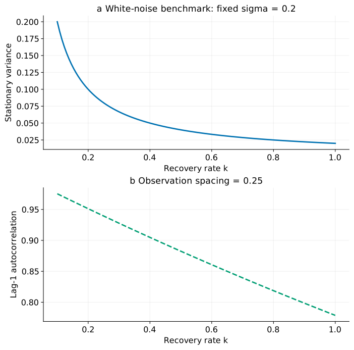
An autocorrelation value is also inseparable from its lag. A value near one at a very short sampling interval can simply mean that consecutive measurements are close together in time. Comparing daily and monthly lag-1 correlations without matching their physical lag confuses the observation schedule with the system.
Variance has its own ambiguity. Increasing raises variance even when does not change. Autocorrelation seems to offer a way around that problem in this particular white-noise model, because its formula does not contain . But that apparent robustness depends on how the noise enters.
The environment also has a memory
Real disturbances often persist. A wet period can last several days; a nutrient input can remain elevated; a temperature anomaly can influence successive observations. Instead of putting independent innovations directly into , give the environment a state of its own:
The environmental driver is an Ornstein–Uhlenbeck process. Its memory time is , while remains the intrinsic recovery time of when the forcing is held unchanged. All variables and times in this experiment are dimensionless.
The coupling coefficient from into has been set to one by the choice of units. That choice is part of the model. An unknown coupling or an unknown sensor gain would introduce additional scaling questions; neither is being silently estimated here.
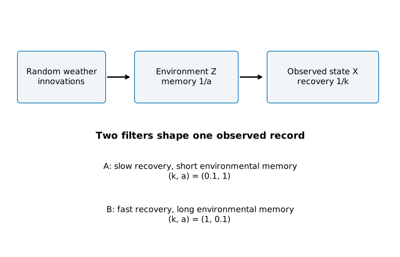
Consider two mechanisms:
| Mechanism | System recovery | Environmental memory |
|---|---|---|
| A: | Slow: recovery time 10 | Short: memory time 1 |
| B: | Fast: recovery time 1 | Long: memory time 10 |
Both have . Mechanism A retains disturbances because the response relaxes slowly. Mechanism B retains them in the observed record because the input keeps pushing, even though the response itself relaxes quickly.
There is a further physical detail: fixing does not fix the variance of . In this model . Lowering makes the environment both more persistent and more variable. The comparison holds the amplitude of fresh innovations fixed, not the environmental variance. This is an explicit modeling choice, and it prevents an overly narrow interpretation of B as “memory changed and absolutely nothing else did.”
The model contains only a stable local response and a stochastic driver. For every positive and tested here, the joint deterministic system has two negative eigenvalues. There is no second ecological state, collapsing population, or threshold crossing built into the experiment.
Calling A “slow recovery” is therefore exact; calling it “an imminent ecosystem collapse” would add information the model does not contain. The first claim concerns a local slope. The second would require a nonlinear mechanism, a changing control parameter, and an event definition.
Two mechanisms, the same observed process
Frequency space makes the ambiguity unusually clear. A linear relaxation equation acts as a filter: slowly varying inputs pass through differently from rapidly varying inputs. At angular frequency , the environment contributes a factor and the system contributes .
Their product gives the transfer function from the white-noise innovations to the observable:
Using the convention that covariance is the inverse Fourier transform with factor , its two-sided power spectral density is
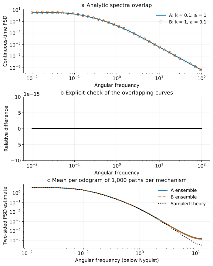
The two factors multiply. Exchanging and leaves their product unchanged. Thus A and B have the same spectrum at every frequency, rather than merely sharing one selected summary.
At low frequencies, both filters can contribute substantially to long excursions. At high frequencies, their combined attenuation produces an decay. The spectrum can reveal the presence of two characteristic rates, but the ordering of those rates in this cascade is absent from the observed output.
What exactly does “the same” mean? Both stationary outputs have mean zero and are Gaussian processes. A Gaussian process is determined by its mean and covariance function. Equal spectra imply equal covariance functions, and therefore equal joint distributions for every finite collection of observation times.
In particular, the vector has the same distribution under A and B for any fixed times. This is stronger than equal variance, equal lag-1 correlation, or an inability to distinguish two finite datasets in one statistical test.
It does not require two independently simulated paths to lie on top of each other. Independent draws from the same distribution will usually look different. Equality of laws describes which patterns occur with which probabilities; it does not prescribe identical random outcomes.
Nor does a simulation prove the equality. The argument rests on the transfer function and Gaussian assumptions. Simulation checks that the implementation is consistent with that argument and shows how an analyst encounters the result through finite records.
Checking the result without a spectrum
The same conclusion appears in the stationary moments. Write
Balancing these quantities gives three equations:
Solving them yields
Only the last quantity is symmetric in the two rates. This is important: the joint process is not observationally equivalent once is measured with a known scale. Information capable of separating the mechanisms exists, but the original sensor does not collect it.
The normalized autocorrelation of is
The apparent singularity at is removable. Taking the limit gives
This equal-rate case matters in practice. A formula that divides by without handling the limit can produce numerical failure exactly where the two mechanisms meet. Here it provides a useful analytic control, and it is included in the experiment.
The output covariance can also be understood as the result of two exponential filters in series. The order of scalar convolution does not change the final filter. However, the intermediate state and the response to an intervention applied between those filters do depend on which filter is where. That distinction is why passive equivalence and different intervention responses can coexist.
What the finite-record experiment shows
The parameter grid uses five separate stationary conditions,
Each condition has 1,000 independent paths, observed 2,048 times at interval . The elapsed time from the first observation to the last is 511.75. Fresh random streams are used for every ensemble.
The grid is not a time-varying trajectory. Moving across its columns does not represent a lake gradually approaching a threshold. Concatenating the records would create changes in the data-generating process that are absent from the stationary proof.
The simulator samples the linear stochastic system exactly at the observation times. In matrix form, with ,
If is the stationary covariance matrix, the innovation covariance is
The initial state is drawn from the stationary Gaussian law with covariance . There is no artificial warm-up transient to be confused with changing resilience. Exact sampling removes time-stepping bias for this linear model; it does not remove finite-sample uncertainty.
Independent checks compare the analytic covariance with the continuous Lyapunov equation, integrate the spectrum back to the variance, and compare the covariance formula with a matrix-exponential calculation. Two half-steps reproduce one full step in both transition and innovation covariance. The equal-rate case is tested alongside the other pairs.
The stationary values shared by A and B are:
| Variance of | Lag-1 autocorrelation | |
|---|---|---|
| 0.1 | 0.181818 | 0.997144 |
| 0.2 | 0.083333 | 0.994337 |
| 0.4 | 0.035714 | 0.988862 |
| 0.7 | 0.016807 | 0.980988 |
| 1.0 | 0.010000 | 0.973501 |
The large autocorrelations partly reflect the short observation spacing relative to both filters. They are not stand-alone numerical thresholds for danger. In particular, an analyst applying the white-noise formula here would obtain an apparent rate that generally equals neither of the two physical rates.
For , the average known-zero-mean second moment was 0.182640 under A and 0.181439 under B. Their Monte Carlo standard errors, calculated across independent paths, were 0.001239 and 0.001207 respectively. Both are consistent with the population variance 0.181818.
Across all ten ensembles, the largest absolute standardized discrepancy of this second-moment estimate from theory was about 1.15 Monte Carlo standard errors. The computation checked a predeclared tolerance of five standard errors. This is an implementation consistency check, not evidence that the mechanisms are scientifically distinguishable or an estimate of a forecasting method’s accuracy.
Why the sample variance sits below theory
A real analyst rarely knows the population mean exactly. For each path, the plotted estimator subtracts its own sample mean:
Because the true mean is zero,
Positive serial correlation makes the second term appreciable. A long, slowly wandering excursion shifts the record’s estimated mean; subtracting that mean removes part of the low-frequency variability we wanted to measure.
Writing the covariance as , the exact mean-estimation penalty is
At , the expected demeaned variance is about 0.174160, although the population variance is 0.181818. The simulated ensemble means are 0.175033 and 0.173840. This discrepancy has a predictable finite-record explanation; it need not signal a faulty simulation or a different ecological mechanism.
Changing the denominator from to only applies the usual independent-data correction. It does not generally cancel the contribution from correlated observation pairs. Likewise, collecting measurements more frequently over the same total duration is not equivalent to observing more independent recovery episodes.
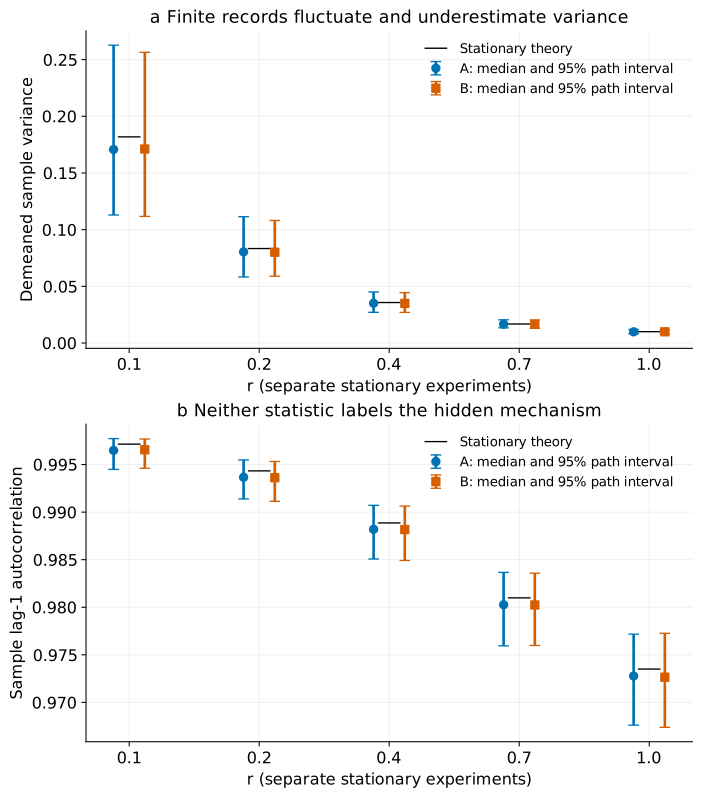
The autocorrelation estimator uses the adjacent centered-product sum divided by the full centered sum of squares. Its finite-record behavior depends on that definition, including the missing last adjacent product. It is not an unbiased estimate of the population correlation. Both mechanisms use the same estimator, so the comparison is fair without pretending that its median must equal theory.
For the spectrum, an additional distinction matters. The continuous-time analytic curve and the spectrum of a sampled sequence are not identical objects. Sampling folds contributions from higher frequencies into the observed frequency band. The ensemble periodograms are therefore compared with the spectrum implied by the exact sampled covariance. Finite record length still introduces leakage; averaging paths reduces random spectral scatter, not that deterministic finite-window effect.
Why a stronger AI cannot manufacture the missing label
Suppose a classifier receives a full record of and must decide between these two fixed mechanisms. Under equal prior probabilities and the stationary design, the likelihoods are identical:
Bayes’ rule therefore leaves the posterior odds equal to the prior odds. With equal priors, optimal expected classification accuracy is 50%. This is an analytic consequence of the experimental setup; no neural network was trained to produce a 50% benchmark result.
The argument does not depend on the classifier’s architecture. A transformer, a recurrent model, or a hand-designed indicator receives a random object with the same law under both labels. Applying a function to that object cannot make its two distributions different.
Training can nevertheless produce confident predictions. Imagine a simulator that labels every low-frequency record “weak recovery” while never generating persistent forcing. A model can learn that association accurately within the training distribution. Its confidence then reflects a restricted set of possibilities supplied by the simulator.
When the deployment environment admits the second mechanism, confidence alone does not establish identification. The missing question is whether the training distribution included scientifically plausible alternatives with similar observable behavior. A held-out split of the same restricted simulator would not answer that question.
The same caution applies to apparently helpful features. Variance, autocorrelation at several lags, power in low-frequency bands, and wavelet coefficients are all transformations of the original record. Under the exact equivalence here, none supplies a new physical label.
That does not make them useless. They can estimate the observed process more accurately, support forecasts of , reveal departures from the assumed model, or help compare hypotheses that are not observationally equivalent. The limitation concerns the particular question “which of these two rates belongs to intrinsic recovery?”
In fact, forecasting and mechanism identification can separate cleanly. If A and B imply the same joint law for the observed past and future, they also imply the same conditional forecast distribution for future given past . A model can forecast the next readings well while remaining unable to identify the mechanism.
This is a useful lesson for AI for science. Prediction error is evidence about the prediction task. It becomes evidence about a hidden mechanism only when the observation model, hypothesis space, and identification conditions connect those tasks.
What a longer record would still accomplish
More observations can reduce uncertainty about variance, correlation shape, and the unordered pair of characteristic rates. They can make the two spectral bends easier to estimate if both fall within the observable frequency range.
But locating two rates is not the same as assigning their physical roles. Even with arbitrarily precise output statistics, the likelihood retains its exchange symmetry. Reporting only one optimum can hide another equally supported interpretation.
An optimizer may select one mode because of its initial values or parameter bounds. A posterior sampler may explore only one mode because transitions between modes are difficult. Neither computational behavior creates scientific evidence favoring that mode.
Ordering the rates, for example imposing , is a legitimate parameterization of an unordered pair. Calling the smaller rate “ecosystem recovery” then requires an additional assumption that the environment relaxes faster. That assumption should come from external knowledge, not from the output record that cannot distinguish the order.
Which additional observations change the answer?
There are two especially direct ways to break the symmetry: observe the driver, or perturb the system at a known point in the causal chain.
If can be measured with an understood observation model, its covariance is no longer symmetric under the parameter exchange. Its own autocorrelation decays at rate . Having estimated the environmental time scale, an analyst has information for assigning the other observed time scale to the response.
In an ideal noise-free continuous record of both variables, the equation supplies a direct relation for . Real discrete and noisy data require joint state-space estimation; simply differentiating a noisy sensor record can amplify measurement noise badly.
A rain gauge is not automatically a measurement of . The effective driver in the lake could combine runoff, nutrient transport, temperature, and delayed catchment response. A useful sensor must measure a variable whose relationship to the modeled input is physically understood.
Sensor placement should therefore follow the ambiguous mechanism. Collecting a second copy of the same water-quality indicator can reduce instrument error, but it does not necessarily reveal whether memory sits in the environment or in the ecosystem. Measuring a forcing-related variable can be more informative even if its readings are less frequent.
The second possibility is a known initial displacement of that leaves unchanged. Compare perturbed and unperturbed systems exposed to the same subsequent forcing. Their difference obeys
so
The environment cancels from this difference because the intervention did not change it. An ensemble experiment with matched initial environmental distributions and independent zero-mean forcing has the same mean-response difference, although individual noisy paths do not cancel exactly.
Under A the response decays with time constant 10; under B it decays with time constant 1. That distinction was absent from the passive law of , but it appears in the intervention response because the intervention targets the state between the two filters.
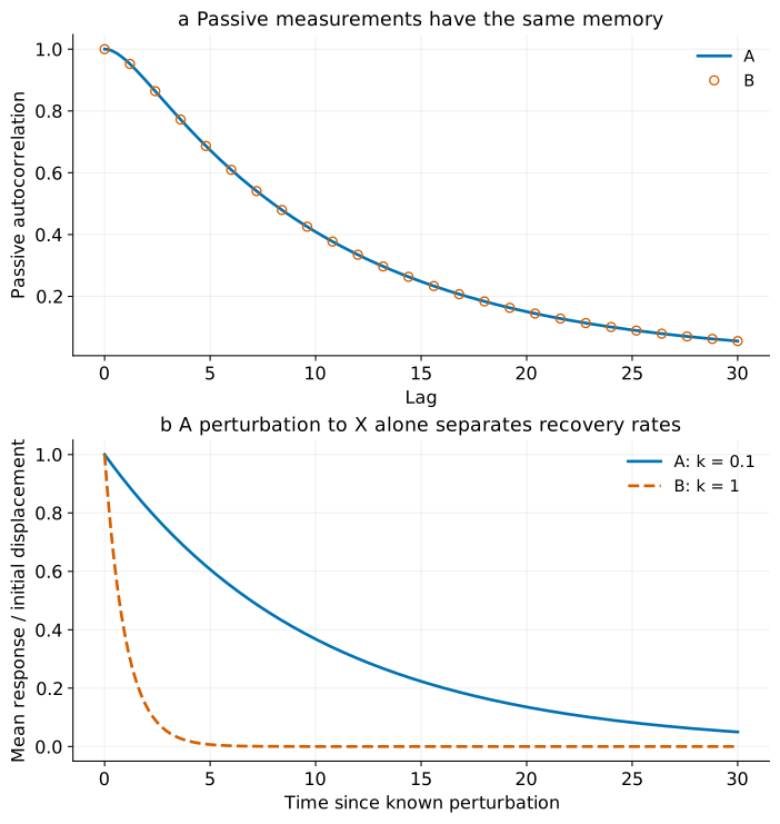
This thought experiment does not recommend perturbing an actual lake. A controlled microcosm, an independently justified natural experiment, or an existing management intervention with suitable observations might offer relevant information. Whether any of these represents the local dynamics of interest needs its own evidence.
A natural storm is particularly easy to misinterpret as the required experiment. It may change for a prolonged period rather than create an isolated displacement of . Fitting an exponential to the subsequent trajectory can then estimate the combined response to continuing forcing instead of intrinsic recovery.
The intervention amplitude also matters. The derivation uses a linear local response. A large manipulation can alter background conditions, activate nonlinear feedbacks, or change the very rate being measured. Repeated small perturbations with stable conditions address a different scientific question from a single large disturbance.
Even in an ideal design, estimating a decay rate requires observations over useful lags. If all measurements occur long after recovery has finished, the signal is gone. If they cover only a tiny fraction of the recovery time, different decay rates may be practically hard to separate despite being theoretically identifiable.
From a statistical change to a scientific explanation
There are several steps between detecting a change in a monitoring record and claiming that a tipping point is approaching. The measured process might change because recovery changes, because forcing changes, because the sensor changes, or because the preprocessing changes.
The 2025 perspective by Rietkerk and colleagues discusses both theoretical and statistical ambiguities in early-warning interpretation, including slowing without the tipping behavior of interest and alternative explanations for detected indicators. It motivates comparing plausible mechanisms rather than equating a significant trend with a tipping probability. Rietkerk et al., 2025.
Our exchange-symmetric example isolates one of these questions in a form that can be solved exactly. It does not reproduce that paper’s climate experiments, assess any named Earth-system component, or imply that all environmental data are equally uninformative.
A separate problem arises when we select records because something dramatic happened at their end. Boettiger and Hastings show how conditioning on observed transitions can bias assessments of common warning statistics. A retrospective pattern before a selected collapse need not demonstrate prospective forecasting ability. Boettiger and Hastings, 2012.
The present experiment avoids that selection by retaining every simulated path and by defining no collapse event. Consequently, it does not report false-alarm rates, missed-collapse rates, or warning lead times. Those quantities require an event definition and a prospective evaluation design that this stationary study does not contain.
A future forecasting experiment would need both transition and non-transition cases sampled according to a stated population. Its processing choices would need to use only information available when an alarm is issued. Thresholds would be calibrated separately from evaluation, and performance would be reported at a defined forecast horizon.
That future experiment should also contain alternative drivers, not merely multiple random seeds of the same tipping mechanism. Otherwise it tests robustness to noise within a preferred explanation while leaving the more consequential ambiguity untouched.
What to ask of the next monitoring campaign
Return to the hypothetical lake. The team should first establish what changed in the measured record and over which physical time scales. A stable sampling schedule, documented sensor changes, and a transparent treatment of seasonality are prerequisites for comparing those records meaningfully.
Next, the team can write down competing explanations before selecting a forecasting method. If slow recovery and persistent forcing are both plausible, a useful study asks what each would predict for an additional environmental measurement or an independently characterized perturbation.
The practical target is a contrast: an observation expected to behave differently under the alternatives. More precise measurements of an identical prediction can be valuable for monitoring, but they are an inefficient way to choose between those alternatives.
This distinction changes how uncertainty is communicated. An honest report can say that variability and persistence increased, quantify the uncertainty in those estimates, and explain why intrinsic recovery has not yet been separated from environmental forcing. It can then identify the extra measurement most likely to resolve the question.
Scientific uncertainty does not determine a management decision by itself. A decision can depend on the consequences of delayed action, the costs of monitoring, and measures that are beneficial under multiple plausible explanations. Those are additional inputs, not numbers hidden inside an autocorrelation coefficient.
The model also suggests a constructive use for AI: help integrate measurements of the driver and response, design informative observations, or estimate complex likelihoods under clearly stated alternatives. The value comes from connecting computation to information that distinguishes mechanisms.
Conclusion
An observed system can remember because its own recovery is slow, because its environment is persistent, or because both mechanisms contribute. In the stationary Gaussian cascade studied here, exchanging the two relaxation rates leaves the entire observed process unchanged.
The simulation makes finite-record uncertainty visible; the mathematics explains why more accurate output statistics cannot assign the hidden labels. A known perturbation or a suitable measurement of the driver changes the information available and can separate the rates.
For environmental modeling, the useful question is therefore not only whether an indicator rises. It is whether the observations distinguish the mechanism that would make that rise scientifically meaningful—and what we should measure next if they do not.
References
- Scheffer, M., et al. (2009). Early-warning signals for critical transitions. Nature, 461, 53–59.
- Rietkerk, M., Skiba, V., Weinans, E., Hébert, R., and Laepple, T. (2025). Ambiguity of early warning signals for climate tipping points. Nature Climate Change, 15, 479–488.
- Boettiger, C., and Hastings, A. (2012). Early warning signals and the prosecutor’s fallacy. Proceedings of the Royal Society B, 279, 4734–4739. Author manuscript.