
A traffic simulation can conserve every vehicle, keep density inside its admissible range, and still report a queue too late. The problem is not necessarily a coding bug. A shock-capturing method represents an abrupt traffic front over a finite number of cells. If an operational rule says that congestion has arrived when density at a sensor first exceeds a threshold, a smeared front changes the reported crossing time. The same smearing changes any queue length or accumulated congestion measure defined by another threshold.
There is a second, more treacherous effect. A global cell-average error can look exceptionally small when the exact discontinuity happens to land on a grid boundary at the final reporting time. That alignment says almost nothing about how accurately the numerical front crossed a sensor earlier. In the frozen example studied here, the coarsest Godunov solution has a final cell-average error of only , yet it reports the threshold arrival time units late. Refining once to 100 cells makes the final error larger, , even while the arrival delay is cut in half.
That is why this project retains a scientific null. Its predeclared Phase-1 criterion required strictly refining final error for Godunov and Rusanov across all four grids. Both checks failed, so the final-norm criterion is not supported. Nothing was tuned after seeing the anomaly, and no failed criterion was deleted. The useful conclusion is not that the solvers are invalid. It is that a single global norm, sampled at a single fortunate time, is not an adequate operational validation of a moving discontinuity.
The benchmark is deliberately synthetic and dimensionless. It contains no road geometry, detector feed, vehicle trajectory, calibrated fundamental diagram, travel-time validation, safety threshold, or policy intervention. Words such as “queue,” “arrival,” and “congestion area-time” name mathematical functionals of the simulated density. They must not be mistaken for observed vehicle delay. Within that boundary, the exact solution makes the measurement problem transparent enough to analyze line by line.
What the traffic experiment found
The central results can be read directly from the model, error definitions, and four figures.
| Question | Result | Why it matters |
|---|---|---|
| Model | Scalar LWR with | One dimensionless concave flux, not an empirically calibrated fundamental diagram. |
| Initial states | , at | One backward-moving Riemann shock. |
| Domain and horizon | , | One closed numerical experiment with fixed boundary states. |
| Exact speed | The discontinuity reaches the fixed sensor at . | |
| Operational threshold | A declared numerical event definition, not a statutory congestion standard. | |
| Numerical design | Three schemes, , CFL | Twelve conservative finite-volume cases under a matched grid ladder. |
| Invariant checks | All finite, bounded, conservative, and observed | Necessary numerical safeguards held; they do not by themselves prove accuracy. |
| Main comparison | NULL / FAIL | Strict final- refinement failed for Godunov and Rusanov and remains failed. |
The distinction in the last column is the core interpretive rule. A conservation residual near machine precision shows that the discrete accounting closes. It does not show that a sensor event is timely. A small final norm describes a particular state comparison, not the complete history of a moving threshold crossing.
Why prior work changed the question
The starting idea suggested that a modified-equation view might reveal how a traffic solver “invents” congestion through artificial viscosity. That is a reasonable teaching motivation, but it is not a defensible novelty claim. The relevant mathematical and transportation literature is much older and broader than this experiment.
Lighthill and Whitham formulated kinematic waves for long crowded roads in 1955 (DOI), and Richards independently developed the highway shock-wave model in 1956 (DOI). Godunov’s 1959 construction supplied the conservative Riemann-solver framework used by the baseline here (official MathNet record). Ansorge later made the entropy condition explicit in traffic-flow computation (DOI).
Daganzo’s cell-transmission model connected a practical discrete traffic representation to hydrodynamic theory in Part I (DOI) and extended it to networks in Part II (DOI). Jin and Zhang treated an inhomogeneous LWR model as a resonant nonlinear system and used a Godunov formulation (DOI). Daganzo’s variational formulation (DOI) and the analytical, grid-free solutions of Mazaré and colleagues (DOI) show that grid-based finite-volume output is not the only available reference language.
High-resolution shock computation is also established territory. Harten’s high-resolution schemes for hyperbolic conservation laws (DOI) and the central schemes of Kurganov and Tadmor (DOI) long predate this benchmark. Friedrich, Kolb, and Göttlich provide a more recent Godunov-type traffic-flow comparison in a non-local LWR setting (DOI).
The literature verdict is REFRAME. The evidence cannot support “we discovered numerical diffusion in traffic flow,” “we invented a better shock solver,” or “we derived a new universal modified-equation coefficient.” The honest local question is narrower:
For one fixed backward LWR shock, can final shock-grid alignment make a cell-average refinement criterion misleading while fixed sensor-arrival and threshold-defined queue metrics still expose numerical bias?
This question is a controlled extension of established theory. Its value comes from comparing an exact solution, a sensor definition, several error functionals, and an unchanged decision rule while retaining the failed final-norm result. It does not depend on pretending that mature theory is novel.
The exact LWR problem
The scalar Lighthill–Whitham–Richards conservation law is
where is a dimensionless density and the frozen Greenshields flux is
The flux is concave, reaches its maximum at , and is defined here only as a canonical test function. No units are attached to density, distance, time, or flow. The initial condition is a Riemann jump at :
Because for a concave flux, the entropy solution is a shock rather than a rarefaction. The Rankine–Hugoniot speed is the flux jump divided by the density jump:
Here
so
The negative sign means the dense state propagates upstream, toward smaller . The exact shock position is
At the final time , it is at . A sensor is fixed at , so the exact front reaches it when
Those two exact locations— at the event and at final time—are the geometric skeleton of the test. They let us distinguish error in the final cell averages from error in the time at which a thresholded sensor sees the front.
Exact cell averages are not point samples
Discontinuous solutions require care when defining error. A numerical finite-volume value represents the average density over a cell, not the value at its center. The correct final reference is therefore the exact average of the step function over every numerical cell.
For a cell of width , the exact reference is
If the shock lies outside the cell, this average is simply or . If the shock cuts the cell, the average is the length-weighted mixture of the two states. That is the appropriate reference for
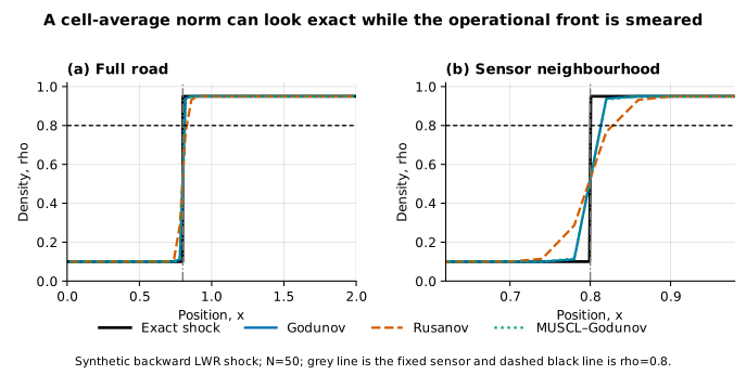
At , the exact shock lies at . On the grid over , , and is a cell boundary in the implemented mesh convention. The first-order Godunov update happens to reproduce the final cell-average step to almost floating-point precision in this case. The resulting error, , is real. It is not a corrupted file and not a plotting mistake.
But it is a geometric coincidence. The front was numerically smeared while travelling. A thresholded sensor at did not see density at the exact time ; the interpolated numerical event occurred at . The final alignment rewards the state norm for being evaluated at a fortunate location and time, while the earlier event metric retains the travel-history bias.
This is not a paradox. Two diagnostics ask two different questions:
- The final norm asks how close all cell averages are to the exact state at .
- The arrival delay asks when one interpolated sensor trajectory first crossed a fixed density threshold.
Neither is intrinsically superior. The mistake would be to use the first as a complete substitute for the second when the intended output is an event time.
Three schemes under one frozen protocol
The experiment compares Godunov, Rusanov, and MUSCL–Godunov finite-volume schemes. Each uses the same domain, boundary states, horizon, CFL number , and grid ladder . This matched design is important: changing the time-step policy, boundary treatment, reconstruction limiter, or event interpolation between schemes would confound the diagnostic.
For a conservative cell update,
the numerical flux determines how information crosses a cell interface. Godunov uses the exact scalar Riemann flux for the concave . Rusanov uses a central average plus dissipation proportional to a local speed bound. MUSCL–Godunov reconstructs limited piecewise-linear interface states before applying the Godunov flux, with twice as many recorded flux evaluations in this implementation.
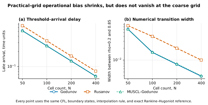
One might expect the nominally higher-resolution reconstruction always to beat a first-order method. The frozen result warns against that simplistic ranking. For this single discontinuity-dominated Riemann case, Godunov and MUSCL–Godunov produce nearly coincident operational curves. Their arrival delays are both about , their final queue errors are and , and their transition widths are and . This does not prove equivalence; it only reports that the reconstruction provides no visible advantage on these declared metrics and settings.
Rusanov is more diffusive in the same design. At , its arrival delay is , compared with for Godunov; its transition width is , compared with . At , those figures decrease to and , but they remain above the Godunov values. This is a conditional comparison for one flux and one shock. It is not a universal league table for traffic solvers.
Operational diagnostics must be declared, not improvised
The arrival event is defined before running the grid study. At the fixed sensor , the numerical density is interpolated in time, and arrival is the first upcrossing of
The arrival error is
The sign matters: every frozen case is late. A method that smears a high-density state into a gradual ramp may cross a high threshold only after the exact discontinuity has passed the sensor.
The transition width is the spatial distance between the locations where the final profile crosses and . It is a direct description of numerical smearing. The two values are not physical traffic standards; they are fixed diagnostic levels spanning most of the jump from to .
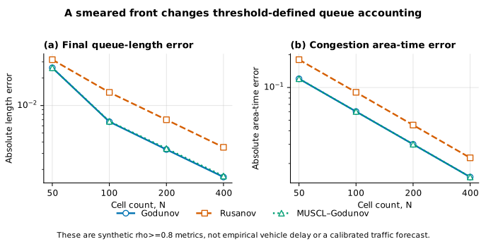
Two additional functionals translate the density field into threshold-defined bookkeeping. The final queue length measures the spatial extent classified as congested at . The congestion area-time integrates that classified extent over the whole horizon. Their exact reference values are and in the dimensionless experiment. The code evaluates numerical counterparts consistently on every grid and reports signed and absolute errors.
These metrics are operational only in a mathematical sense. The “queue” is not a counted line of vehicles; the threshold is not estimated from a detector; the area-time is not a welfare or emissions measure. Their purpose is to expose how a blurred interface changes downstream functionals even when mass conservation is exact.
What the twelve cases actually show
For Godunov, grid doubling reduces the arrival delay from to , , and . The absolute final queue-length error falls from to , , and . The absolute congestion area-time error falls from to , , and . Transition width shrinks from to , , and .
Rusanov follows the same broad refinement pattern but with larger errors: arrival delays , , , ; queue errors , , , ; area-time errors , , , ; and transition widths , , , .
MUSCL–Godunov closely tracks Godunov: arrival delays , , , ; queue errors , , , ; area-time errors , , , ; and transition widths , , , .
Several patterns deserve precise wording.
First, every scheme shows regular improvement in the fixed arrival metric under each grid doubling. The delay is approximately halved. Second, transition width also shrinks regularly. Third, the threshold-defined queue functionals improve, though the first Godunov queue-length reduction is especially large because geometry affects the final threshold intersection. Fourth, Rusanov is consistently more diffusive than Godunov on these metrics. Fifth, MUSCL reconstruction does not materially separate itself from Godunov in this test.
None of those statements changes the predeclared global criterion. It requires final error to decrease strictly at every refinement for both Godunov and Rusanov. Neither sequence does.
Why the final norm failed its test
The Godunov final sequence is
The first step increases because receives the alignment windfall. The Rusanov sequence is
It also increases at the first step before entering a regular refinement regime. Neither Godunov nor Rusanov therefore satisfies the required strictly decreasing four-grid sequence, so the declared final-norm criterion fails.
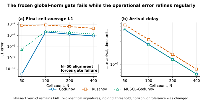
It would be easy to make the result appear favourable. The comparison could start at , move the final time so the shock no longer aligns, weaken “strictly monotone” to “eventually decreasing,” change the error to point samples, or replace the primary criterion with arrival delay after inspecting the output. Each change might define a sensible new experiment. None changes the result of this fixed comparison.
Preserving the failure is more informative. It documents a counterexample to the implicit assumption that a coarse-to-fine final norm must be monotone in a discontinuity problem. It also shows why validation criteria should be chosen to match the intended output before the numerical results are known.
Reference and invariant checks still matter
Failure of the final-norm criterion does not make the calculation unconstrained. All twelve cases meet several necessary numerical conditions:
- every stored quantity is finite;
- density remains inside the declared interval ;
- the mass-balance residual is at most ;
- every sensor trajectory crosses the event threshold;
- the analytic speed calculation matches to the tolerance;
- exact cell averages are used for the final state comparison.
These checks make the null interpretable. If mass leaked, density became negative, or the event detector missed a crossing, the failed refinement sequence could be an implementation defect. Instead, the consistency checks isolate the failure to the relationship between grid geometry and the chosen final-time norm.
These layers answer different questions:
- Exact reference: establishes the shock and event quantities for the canonical problem.
- Numerical admissibility: establishes conservative, bounded numerical execution.
- Reported errors: quantify state, event, interface, and threshold-functional differences.
- Primary criterion: determines whether the predeclared final-norm claim is supported.
The exact reference and admissibility conditions can hold while the primary criterion fails. That is what happens here: the computation is valid, but the final-norm claim is unsupported.
Why “invents a jam” is a diagnostic title
The title is intentionally provocative but needs a precise translation. The solver does not create mass. It creates a numerical transition layer around an exact discontinuity. A threshold applied to that layer may classify some cells or times differently from a threshold applied to the exact step. The apparent extra or delayed congestion is therefore a joint product of discretization and measurement definition.
Suppose a reporting system records a queue wherever exceeds a threshold . For an exact shock, the classified region changes abruptly at one location. For a smeared profile, there is a finite band in which the classification depends on the chosen threshold. A lower threshold may make congestion appear to extend ahead of the exact front; a high sensor threshold may make arrival appear late. Both effects can occur without violating conservation.
This observation applies beyond traffic. Front arrival in combustion, wetting, epidemics, phase change, reactive transport, and ecological invasion is often extracted from threshold crossings. Whenever the front is numerically diffuse, the solver and the operational definition interact. The transferable lesson is methodological, not empirical: validate the functional that will be reported, not only the field norm that is convenient to compute.
Global norms and event errors answer different questions
An norm is attractive for conservation laws because it is robust to pointwise shock displacement and has strong theoretical relevance. But a small error can arise from different error geometries. A front may be slightly displaced but sharp, correctly located but smeared, or aligned with cell boundaries at the reporting time. These cases can have similar norms and very different event times.
For an ideal step of height displaced by , the continuous difference is roughly . That relation makes a state norm useful for tracking shock position in generic configurations. Yet a finite-volume cell-average comparison introduces mesh geometry, and a thresholded time event adds interpolation and profile-shape dependence. The result is an extreme reminder that a particular discrete norm can receive a cancellation or alignment advantage not shared by the event functional.
This does not argue for abandoning norms. A robust validation panel can include:
- an exact or independently resolved state norm;
- shock-location error;
- threshold-arrival error at declared sensors;
- transition width or total variation diagnostics;
- conservation and admissibility residuals;
- application-specific integral functionals;
- sensitivity to thresholds, sensor positions, final times, and grid offsets in a later, separately declared stage.
The list becomes dangerous if it is assembled after seeing the answer and only favorable metrics are reported. The point of the frozen Phase-1 design is that even an inconvenient norm remains visible.
What this experiment does not establish
The benchmark supports a narrow numerical statement. It does not establish any of the following:
- A real traffic forecast. There are no loop detectors, probe vehicles, cameras, travel times, road capacities, lane changes, incidents, signals, or boundary-demand data.
- A calibrated fundamental diagram. The Greenshields flux is dimensionless and chosen for analytic transparency.
- A policy or safety conclusion. The threshold values are numerical definitions, not legal, engineering, or operational standards.
- A universal scheme ranking. One Riemann shock at CFL cannot rank methods across smooth waves, interacting shocks, rarefactions, networks, sources, non-local fluxes, or heterogeneous roads.
- A new convergence theorem. The study records four-grid behavior; it proves no asymptotic rate.
- A derived modified-equation coefficient. No general artificial-viscosity formula is fitted or claimed.
- The superiority of MUSCL reconstruction. Its near-coincidence with Godunov here is a case result, not a method verdict.
- That global norms are useless. The result shows incompleteness for event-focused validation, not irrelevance.
Those limitations are part of the result rather than boilerplate. They prevent a clean synthetic counterexample from being inflated into a transportation claim.
Why the null is credible
An independent calculation returned the same twelve case results, including the near-zero coarse-grid norm, the arrival delay, and both non-monotone refinement sequences. Separate analytic and numerical comparisons recover the shock speed and exact cell-average reference, keep density within bounds, close the mass balance, and detect every declared crossing.
Every comparison in this article uses , the time at which the defining mesh alignment occurs. A different final time would alter that geometry and answer a different question, so the interpretation is tied to the stated horizon rather than extrapolated to arbitrary times.
The null is therefore not explained by lost mass, negative density, a missed event, or a point-sample reference. It comes from a known geometric mechanism: the final shock happens to coincide with a boundary of the coarse mesh while the earlier sensor crossing does not share that phase. Repeating the calculation confirms the numbers; the exact solution explains them.
The two observables interrogate different geometries. The final norm aggregates cell averages over the whole road, while the arrival time depends on one local threshold crossing. Exact alignment can cancel the first error without cancelling the second, which is why conservation and a small terminal norm cannot substitute for direct event validation.
A better validation question
The most productive change is not to ask, “Which scheme has the smallest number?” It is to ask, “Which numerical property must be accurate for the decision or scientific statement we intend to make?”
If the output is total vehicle count, conservation deserves priority. If it is density reconstruction, state norms and spatial structure matter. If it is the time a front reaches a detector, the event definition and interpolation require direct verification. If it is a queue duration above a threshold, sensitivity to that threshold and to numerical transition width becomes part of the validation problem.
This functional-first view avoids proxy substitution and metric shopping. Proxy substitution validates a convenient state norm and then assumes every downstream metric is valid. Metric shopping computes many summaries after the run and highlights whichever support the desired claim. Fix the intended functional, retain exact-reference and admissibility conditions, and specify what constitutes success before computation.
For teaching, the alignment case is especially useful because the contradiction is visible without advanced machinery. The coarse grid appears “perfect” in one number and clearly late in another. Students can trace both results back to exact geometry rather than treating them as mysterious software behavior.
Threshold sensitivity deserves its own experiment. The exact step crosses every intermediate density threshold at the same instant, but a numerical ramp crosses low thresholds before high ones. A later study could fix several thresholds in advance and plot event time against threshold for each grid. The spread of those times would quantify how much of the reported arrival depends on the operational definition rather than the front location alone.
Grid phase is another independent axis. Shifting the initial discontinuity by a fraction of one cell, or shifting the reporting time while keeping the dynamics unchanged, moves the exact front through different positions inside a cell. Reporting the distribution of errors over those phases would distinguish a method’s typical behaviour from the fortunate alignment seen here. One phase cannot supply that distribution.
Shock speed should vary as well. A fixed spatial displacement becomes a time error after division by the front speed, so the same transition width can produce very different arrival delays for slow and fast shocks. A follow-up spanning several left and right states would separate this kinematic amplification from the diffusion introduced by each scheme. The present speed supplies one transparent example, not a general conversion between grid error and operational delay.
What a responsible next stage would test
The current evidence should not be expanded by silently adding more favorable cases. A separate Phase 2 could freeze a broader robustness design with several deliberate axes:
- shift the initial discontinuity relative to the mesh;
- vary final time so the exact front samples different grid phases;
- move sensors and change declared thresholds;
- include rarefactions and shock interactions;
- compare smooth and discontinuous initial conditions;
- vary CFL under matched work or accuracy budgets;
- add independent variational or grid-free references;
- evaluate flux and reconstruction choices under declared work accounting;
- separate interpolation error from evolution error;
- report distributions across grid offsets rather than one fortunate phase.
An empirical traffic study would require a different evidence layer altogether: a real site, units, detector metadata, data-quality rules, calibration and holdout periods, uncertainty in demand and capacity, and a predeclared link between simulated functionals and measured outcomes. Nothing in this synthetic Phase 1 substitutes for that work.
The modified-equation idea could also be revisited, but only with an explicit derivation and a claim matched to what is proved. Fitting an “effective viscosity” after observing four curves would not establish a general coefficient. A serious analysis would distinguish scheme, flux, limiter, solution regime, grid, and time-step dependence, and it would test predictions on held-out configurations.
Conclusion
The headline result is intentionally uncomfortable: the coarsest Godunov grid is almost exact in the final cell-average norm and still late at the sensor. The next grid has a worse final norm and a better arrival time. Rusanov shows its own non-monotone first refinement. The predeclared final-norm criterion therefore fails. At the same time, conservation and boundedness hold, the reference calculations remain consistent, an independent repeat returns the same values, and the operational errors improve with refinement.
That combination is not a broken study. It is the study’s contribution. It demonstrates, in one exact synthetic case, why numerical validation needs a portfolio of declared diagnostics tied to the intended output. A solver can preserve mass without preserving an event time. A norm can be small for a geometric reason that does not benefit an operational functional. A higher-resolution label does not guarantee a visible advantage in every discontinuity-dominated test. And a null result can teach more than a retuned success.
So when the title says that a traffic solver “invents a jam,” the precise meaning is modest: numerical smearing changes threshold-defined congestion bookkeeping. It does not mean that simulated vehicles appeared from nowhere, and it does not describe a real road. The honest lesson is broader and more durable: whenever a scientific conclusion depends on a moving front, validate the front-dependent conclusion directly.