當交通求解器製造出一場塞車

一個交通模擬可以做到車輛總量完全守恆、密度從不超出容許範圍、每一步計算都有限，卻仍然把「塞車到達感應器的時間」報遲。這不一定是程式錯誤。捕捉激波的數值方法要在有限網格上表示一個突然跳躍，因此通常把理想的不連續面攤成幾個 cell 寬的過渡層。若操作規則把「感應器密度第一次超過某個門檻」定義為塞車到達，這層數值模糊便會改變交點時間；若排隊長度及累積擠塞量也由門檻定義，同一過渡層亦會改變那些下游指標。

更危險的是，某個全域 cell-average error 可以因為幾何對齊而顯得異常漂亮。假如精確激波在最後報告時刻剛好落於網格邊界，數值 cell averages 可能與精確 cell averages 幾乎完全相同；但這個巧合沒有回答激波較早之前經過感應器時是否準確。在本文的 frozen example 中，最粗的 $N=50$ Godunov solution 最終 $L^1$ error 只有 $1.37\times10^{-11}$ ，看來接近 floating-point exact；然而同一解把門檻到達時間報遲了 $0.517647$ 個無因次時間單位。把網格加密至 100 cells 後，最終 $L^1$ error 反而增至 $4.60\times10^{-4}$ ，但到達延遲卻減少一半。

因此本專案保留一個科學 null，而不是事後修改規則。第一階段的固定 criterion 要求 Godunov 及 Rusanov 的最終 $L^1$ error 在四層網格上逐次嚴格下降；兩個 checks 都失敗，所以 final-norm criterion 不獲支持。沒有因為圖表不漂亮而移走 $N=50$ ，沒有把 final time 改到另一位置，也沒有在看到結果後換成較有利的 arrival metric。這個負面結果不代表求解器完全無效，而是指出：當研究問題關心移動不連續面的操作事件時，單一時刻、單一全域 norm 並不足以完成驗證。

整個 benchmark 是刻意簡化、完全合成、沒有單位的數值實驗。它沒有道路幾何、loop detector data、probe vehicle trajectories、camera counts、實際 travel time、校準後的 fundamental diagram、事故紀錄、訊號燈、lane-changing model、安全標準或政策措施。本文所說的「queue」、「arrival」及「congestion area-time」只是由合成密度場計算的數學 functionals，不能改寫成真實車輛延誤。在這條清楚界線內，模型足夠精確，讓 shock、sensor event、網格 alignment 與 error metrics 的關係可以逐行核對。

交通實驗發現了甚麼

下表直接列出數值問題、結果及其含義，讓讀者先掌握最重要的比較。

問題	結果	為何重要
模型	$q(\rho)=\rho(1-\rho)$ 的 scalar LWR	單一無因次 concave flux，不是以道路數據校準的 fundamental diagram。
初始狀態	$x_0=1$ 左側 $0.1$ 、右側 $0.95$	一個向上游移動的 Riemann shock。
空間與時間	$x\in[0,2]$ ， $T=6$	一個固定 boundary states 的封閉數值實驗。
精確速度	$s=-0.05$	不連續面在 $t=4$ 到達固定感應器 $x_s=0.8$ 。
事件門檻	$\rho_s=0.8$	預先申明的數值事件，不是法律或交通管理標準。
計算設計	三個 schemes、四層網格、CFL $0.8$	十二個在同一 protocol 下比較的 conservative finite-volume cases。
基本 checks	全部 finite、bounded、conservative、均觀察到 crossing	實作基本一致性通過；這些 checks 本身不等於 accuracy。
主要比較	NULL / FAIL	Godunov 與 Rusanov 的 strict final- $L^1$ refinement 均失敗，而且失敗被保留。

最後一欄是整篇研究最重要的解讀規則。接近 machine precision 的 conservation residual 只證明離散流量核算閉合，沒有證明感應器事件準時。很小的 final norm 只描述指定時刻的 state comparison，不能自動代表移動門檻 crossing。

先行研究怎樣改變了問題

原始構想容易形成一個吸引人的 headline：從 modified equation 看人工黏性如何令 traffic solver「製造」擠塞。作為教學切入點沒有問題，但若聲稱發現一個新現象或新 solver，便忽略了大半個世紀的成熟理論。

Lighthill 與 Whitham 在 1955 年已用 kinematic waves 描述長而擠迫的道路（DOI）；Richards 在 1956 年獨立發展 highway shock-wave model（DOI）。Godunov 在 1959 年提出保守的 Riemann-solver construction，成為本文 baseline 的理論源頭（MathNet 官方紀錄）。Ansorge 其後明確討論 traffic-flow computation 中 entropy condition 的意義（DOI）。

Daganzo 的 cell-transmission model 把 practical discrete representation 與 hydrodynamic theory 接起來；Part I 處理基本動力表示（DOI），Part II 延伸至 networks（DOI）。Jin 與 Zhang 把 inhomogeneous LWR traffic model 寫成 resonant nonlinear system，並使用 Godunov formulation（DOI）。Daganzo 的 variational formulation（DOI）以及 Mazaré 等人的 analytical and grid-free solutions（DOI）亦說明：網格 finite-volume output 從來不是唯一 reference language。

高解析度 shock computation 同樣不是空白領域。Harten 的 high-resolution schemes（DOI）與 Kurganov–Tadmor central schemes（DOI）早已處理 non-oscillatory resolution、numerical diffusion 與 conservation-law fronts。Friedrich、Kolb 與 Göttlich 亦在 non-local LWR 類別中研究 Godunov-type scheme（DOI）。

因此，本地證據不容許「首次發現 traffic numerical diffusion」、「發明更好的 shock solver」、「證明某 scheme 普遍優越」或「推導通用 modified-equation coefficient」。文獻結論是 REFRAME，可辯護的問題應縮窄為：

在一個 fixed backward LWR shock 中，final shock-grid alignment 能否令 cell-average refinement criterion 產生誤導，而固定的 sensor-arrival 與 threshold-defined queue metrics 仍顯示數值偏差？

這是對既有理論的一項受控延伸。價值來自把 exact solution、sensor definition、不同 functionals 與固定 decision rule 放在同一比較中，並保留失敗的 final-norm 結果，而不是把成熟知識包裝成 novelty。

精確的 LWR 問題

本文使用 scalar Lighthill–Whitham–Richards conservation law：

\frac{\partial \rho}{\partial t} +\frac{\partial q(\rho)}{\partial x}=0,

其中 $\rho(x,t)$ 是無因次密度，frozen Greenshields flux 為

q(\rho)=\rho(1-\rho).

此 flux 是 concave，在 $\rho=0.5$ 達最大值。這裡選它是因為解析結構透明，不是因為它已配合某條道路。density、distance、time 及 flow 均沒有實際單位。初始條件在 $x_0=1$ 有一個 Riemann jump：

\rho(x,0)= \begin{cases} 0.1, & x<1,\\ 0.95, & x>1. \end{cases}

對 concave flux 而言， $\rho_L<\rho_R$ 對應 entropy shock，而不是 rarefaction。Rankine–Hugoniot speed 等於 flux jump 除以 density jump：

s=\frac{q(\rho_R)-q(\rho_L)}{\rho_R-\rho_L}.

由於

q(0.1)=0.09, \qquad q(0.95)=0.0475,

所以

s=\frac{0.0475-0.09}{0.95-0.1}=-0.05.

負號代表高密度狀態向較小 $x$ ，即向上游傳播。精確 shock position 是

x_{\mathrm{shock}}(t)=1-0.05t.

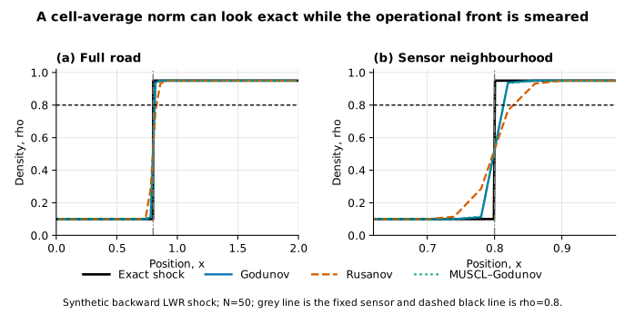
在 final time $T=6$ ，shock 位於 $x=0.7$ 。感應器固定在 $x_s=0.8$ ，因此精確 front 到達時滿足

1-0.05t_s=0.8, \qquad t_s=4.

$x=0.8$ 的 event geometry 與 $x=0.7$ 的 final geometry 是整個測試的骨架。前者讓我們檢查 crossing time，後者讓我們檢查 final state；兩者不應被同一個數字取代。

精確向上游移動的 LWR shock 與三種有限體積密度剖面，左圖顯示整段合成道路，右圖放大固定感應器附近，並標示 queue threshold。 — 精確不連續面與三個 frozen numerical profiles。即使 final cell-average alignment 令全域 norm 異常細小，sensor threshold 仍會對數值過渡層作出不同反應。

為何 reference 必須是 exact cell averages

不連續解的 error definition 不能隨便用 cell-center point samples。Finite-volume state 代表每個 cell 內的平均密度，所以適當的 final reference 應是精確 step function 在相同 cell 上的積分平均。

對寬度為 $\Delta x$ 的 cell $C_i=[x_{i-1/2},x_{i+1/2}]$ ，精確 reference 是

\bar\rho_i^{\mathrm{exact}}(T) =\frac{1}{\Delta x} \int_{C_i}\rho(x,T)\,dx.

若 shock 不在 cell 內，平均值就是 $0.1$ 或 $0.95$ ；若 shock 切穿 cell，平均值則是左右狀態按長度加權的 mixture。本文的 final error 定義為

E_{L^1}(T) =\sum_i \Delta x \left| \bar\rho_i(T)-\bar\rho_i^{\mathrm{exact}}(T) \right|.

在 $T=6$ ，精確 shock 位於 $x=0.7$ 。對 $[0,2]$ 上的 $N=50$ grid， $\Delta x=0.04$ ，而 implemented mesh convention 剛好把 $0.7$ 放在 cell boundary。這個特定案例中，first-order Godunov update 的 final cell-average step 幾乎與 exact averages 重合，因而產生 $1.37\times10^{-11}$ 的 $L^1$ error。這個細小數字來自 final shock 與 cell boundary 的幾何對齊，不代表一般收斂率突然提高。

問題在於它是幾何巧合。front 在移動過程中仍然是數值模糊的。位於 $x=0.8$ 的高門檻 sensor 沒有在精確時間 $4$ 觀察到 $\rho=0.8$ ；經 time interpolation 後，numerical event 是 $4.517647$ 。final alignment 只獎勵最後時刻的 state norm，較早的 event functional 則保留了 travel-history bias。

兩個 diagnostics 根本在問不同問題：

final $L^1$ norm 問：在 $T=6$ ，所有 cell averages 與 exact state 有多接近？
arrival delay 問：一條 interpolated sensor trajectory 何時第一次跨過固定 density threshold？

兩者都可以合理，也都可能有盲點。錯誤不是使用 $L^1$ ，而是在目標明明是 event time 時，把 final $L^1$ 當成完整 substitute。

三種 schemes，共用一個 protocol

實驗比較 Godunov、Rusanov 與 MUSCL–Godunov finite-volume schemes。三者共用 domain、initial and boundary states、final horizon、CFL $0.8$ 、event interpolation 及 $N\in\{50,100,200,400\}$ 的 grid ladder。這個 matched design 很重要；若每個 solver 使用不同 time-step rule、boundary treatment、limiter、threshold 或 sensor interpolation，圖上的差異便同時混入 protocol 差異。

一般 conservative update 可寫成

\bar\rho_i^{n+1} =\bar\rho_i^n -\frac{\Delta t}{\Delta x} \left(F_{i+1/2}^n-F_{i-1/2}^n\right).

Numerical flux $F$ 決定介面兩邊如何交換資訊。Godunov 對 scalar concave flux 使用 exact Riemann flux；Rusanov 使用中央平均再加上與 local speed bound 成比例的 dissipation；MUSCL–Godunov 先以 limited piecewise-linear reconstruction 建立 interface states，再使用 Godunov flux，這個 implementation 的 flux evaluations 約為一階版本兩倍。

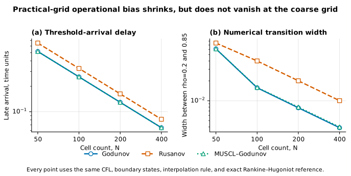
「較高解析度 reconstruction 應永遠勝出」是一個過度簡化的預期。在這個單一、由 discontinuity 主導的 Riemann case 中，Godunov 與 MUSCL–Godunov 的 operational curves 幾乎重合。 $N=400$ 時，兩者 arrival delays 都約為 $0.064706$ ；final queue errors 分別為 $0.001652$ 與 $0.001693$ ；transition widths 為 $0.003905$ 與 $0.004001$ 。這只表示 reconstruction 在本組 metrics 及 settings 沒有帶來可見優勢，不能推廣成兩種方法等價。

同一設計內，Rusanov 較為 diffusive。 $N=50$ 時 arrival delay 是 $0.651582$ ，Godunov 是 $0.517647$ ；transition width 是 $0.074893$ ，Godunov 是 $0.061176$ 。到 $N=400$ 時，它們分別下降至 $0.081450$ 與 $0.010031$ ，但仍高於 Godunov。這是 design-conditional comparison，不是 universal solver ranking。

操作指標必須預先申明

感應器 event 在 grid study 前固定。對 $x_s=0.8$ 的 numerical density trajectory 作 time interpolation，第一次 upcrossing

\rho(x_s,t)=0.8

便是 arrival。Arrival error 定義為

E_{\mathrm{arrival}} =t_{\mathrm{arrival}}^{\mathrm{num}}-4.

正負號有明確意義：十二個 frozen cases 全部是 late arrival。當 high-density state 被攤成 gradual ramp，高 threshold 要等到較大比例的濃密狀態進入 sensor 才會 crossed，因此報告時間可以遲於 exact discontinuity。

Transition width 是 final profile 中 $\rho=0.2$ 與 $\rho=0.85$ 兩個 crossing locations 的空間距離。它直接量度數值 smearing。這兩個密度值不是物理交通標準，只是固定在 $0.1$ 至 $0.95$ jump 內、覆蓋大部分變化幅度的 diagnostic levels。

Godunov、Rusanov 與 MUSCL–Godunov 在四個 cell counts 下的門檻到達延遲及 transition-width refinement，兩個 panel 均以 logarithmic scale 顯示。 — 三個 fixed schemes 的 arrival delay 與 transition width 都隨 grid doubling 規律下降，但預先申明的 global-$L^1$ criterion 仍未成立。

另外兩個 functionals 把 density field 轉成 threshold-defined accounting。Final queue length 計算 $T=6$ 時被分類為 congested 的空間長度；congestion area-time 則把這個 classified extent 在整段 horizon 上積分。Exact references 分別是 $1.3$ 與 $6.9$ 。所有 grids 使用相同定義，並保存 signed 及 absolute errors。

這些 quantities 只是「操作形式上」的指標。Queue 不是實際點算的車列，threshold 不是由 detector data estimate，area-time 亦不是 welfare、emissions 或 safety measure。它們的目的，是顯示 blurred interface 如何改變 downstream functionals，即使 total mass accounting 完全正確。

十二個 cases 的數字

Godunov 的 arrival delay 隨 grid doubling 由 $0.517647$ 降至 $0.258824$ 、 $0.129412$ 及 $0.064706$ 。Absolute final queue-length error 由 $0.025882$ 降至 $0.006650$ 、 $0.003304$ 、 $0.001652$ 。Absolute congestion area-time error 由 $0.120317$ 降至 $0.060119$ 、 $0.030058$ 、 $0.015029$ 。Transition width 則由 $0.061176$ 降至 $0.015719$ 、 $0.007809$ 、 $0.003905$ 。

Rusanov 亦有相似 refinement pattern，但 errors 較大。Arrival delays 是 $0.651582$ 、 $0.325801$ 、 $0.162900$ 、 $0.081450$ ；queue errors 是 $0.031758$ 、 $0.013933$ 、 $0.006989$ 、 $0.003495$ ；area-time errors 是 $0.180281$ 、 $0.090374$ 、 $0.045157$ 、 $0.022571$ ；transition widths 是 $0.074893$ 、 $0.040088$ 、 $0.020061$ 、 $0.010031$ 。

MUSCL–Godunov 緊貼 Godunov：arrival delays 為 $0.517647$ 、 $0.258824$ 、 $0.129412$ 、 $0.064706$ ；queue errors 為 $0.025882$ 、 $0.006720$ 、 $0.003386$ 、 $0.001693$ ；area-time errors 為 $0.120534$ 、 $0.060229$ 、 $0.030115$ 、 $0.015058$ ；transition widths 為 $0.061177$ 、 $0.015883$ 、 $0.008003$ 、 $0.004001$ 。

三種 frozen finite-volume schemes 在四層網格下的 absolute final queue-length error 與 congestion area-time error，兩個 threshold-defined metrics 均以 logarithmic scale 顯示。 — Threshold-defined queue functionals 隨加密而改善，但它們只屬合成數值診斷，不能報告成 empirical vehicle delay 或真實道路擠塞影響。

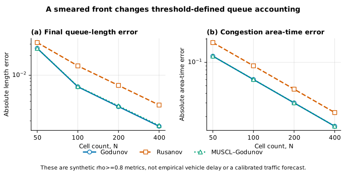
可以用五句精確說法總結。第一，三種 schemes 的固定 arrival metric 在每次 grid doubling 都改善，delay 約減半。第二，transition width 亦規律縮小。第三，兩個 threshold-defined queue functionals 整體改善，雖然幾何位置使部分 first-step ratio 不完全等比。第四，這個設計下 Rusanov consistently 比 Godunov diffusive。第五，MUSCL reconstruction 在本例沒有明顯脫離 Godunov curve。

但這五點都不會改變預先申明的 global criterion。它要求 Godunov 及 Rusanov 的 final $L^1$ 在每一層 refinement 都嚴格下降；兩條 sequence 都沒有做到。

為何 final norm 沒有通過測試

Godunov final $L^1$ sequence 是

1.37\times10^{-11},\quad 4.60\times10^{-4},\quad 1.76\times10^{-4},\quad 8.82\times10^{-5}.

由 $N=50$ 到 $N=100$ 的第一步上升，原因是最粗 grid 得到 alignment windfall。Rusanov sequence 是

6.75\times10^{-3},\quad 8.04\times10^{-3},\quad 4.02\times10^{-3},\quad 2.01\times10^{-3}.

它同樣在第一步上升，其後才進入規律下降。因此 Godunov 與 Rusanov 都不滿足四層網格逐次嚴格下降的要求，預定 final-norm criterion 失敗。

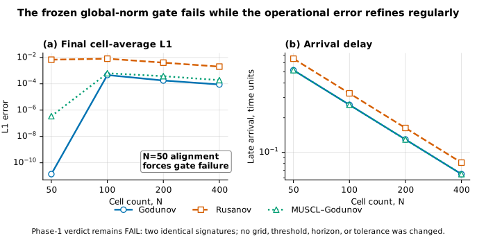
左圖並列 final cell-average L1 error，右圖顯示 threshold-arrival delay，並突出 N 等於 50 的 grid-alignment anomaly 及被保留的 scientific null。 — Null 本身就是結果：coarse-grid final norm 因 alignment 接近零，卻同時有 $0.517647$ late arrival；另一方面，arrival error 在每次 grid doubling 都改善。

要令結果看來通過其實很容易。可以從 $N=100$ 才開始檢查；把 $T=6$ 改成另一時間，令 shock 不再落於 $N=50$ boundary；把「strictly monotone」放寬成「eventually decreasing」；改用 cell-center point samples；或者看到 output 後才把主要判準換成 arrival delay。每一項都可形成一個新的合理 experiment，但沒有一項可以改變這次固定比較的結果。

保留 failure 更有資訊價值。它提供一個清楚 counterexample，說明 discontinuity problem 的 coarse-to-fine final norm 不必 monotone；亦展示 validation criterion 應在知道結果前，按 intended output 選定。

主要判準失敗，基本數值條件仍成立

Final-norm criterion 失敗，不表示數值計算沒有基本約束。十二個 cases 均符合以下必要條件：所有 stored quantities finite；density 維持在 declared interval $[0.1,0.95]$ ；mass-balance residual 不大於 $2.22\times10^{-16}$ ；每條 sensor trajectory 都 crossing event threshold；analytic speed 與 $-0.05$ 在 $10^{-14}$ tolerance 內一致；final state comparison 使用 exact cell averages。

正是這些條件令 null 可解釋。若 model 漏 mass、產生 negative density，或 event detector 根本 miss crossing，那麼 failed sequence 可能只是 implementation defect。現時 exact reference 與 numerical admissibility 都成立，便可把焦點收窄到 grid geometry 與 chosen metric 的相互作用。

四個層次回答不同問題：

Exact reference：確認 canonical problem 的 shock position、speed、event time 及 cell averages。
Numerical admissibility：確認 numerical execution conservative、bounded、finite。
Reported errors：分別量度 state、event、interface width 及 threshold-functional differences。
主要判準：決定預先申明的 final-norm claim 是否獲支持。

Exact reference 與 admissibility 成立時，主要判準仍可失敗。本次正是如此：計算本身有效，原先的 final-norm claim 則不獲支持。

「製造一場塞車」的精確意思

標題刻意有張力，但需要精確翻譯。Solver 沒有創造 mass，也沒有真的把額外車輛放到道路。它創造的是 exact discontinuity 周圍的 numerical transition layer。當 threshold 作用於這一層，部分 cells 或 times 的分類便可能與 exact step 不同。因此 apparent extra congestion、short queue 或 late arrival 是 discretization 與 measurement definition 的共同產物。

假設 reporting system 把 $\rho>\rho_q$ 的位置定義為 queue。對 exact shock，classified region 在單一 location 突然改變；對 smeared profile，則存在有限寬的 band，classification 取決於 $\rho_q$ 。較低 threshold 可能使 congestion 看似伸延至 exact front 前方；較高 sensor threshold 則可能令 arrival 看似遲到。兩個效果都可以在 conservation 完全成立時出現。

這個觀察不只適用於 traffic。Combustion front、wetting front、epidemic wave、phase change、reactive transport、ecological invasion 及 tumour boundary 都常由 threshold crossing 提取 event time 或 extent。只要 numerical front 有 diffusion，solver 與 operational definition 就會互相影響。可轉移的 lesson 是方法論：驗證最後要報告的 functional，而不只驗證最方便計算的 field norm。

Global norm 與 event error 回答不同問題

$L^1$ norm 在 conservation laws 中非常重要，因為它對 pointwise shock mismatch 較穩健，亦有清楚理論意義。不過，小 $L^1$ error 可以來自不同 error geometry。Front 可以位置稍錯但非常 sharp；位置正確但很 smeared；或者只在 reporting time 剛好與 cell boundary 對齊。這些 cases 可能有近似 norm，卻有很不同 event times。

對高度 $\Delta\rho$ 、位置偏移 $\delta x$ 的 ideal steps，continuous $L^1$ difference 大約是 $|\Delta\rho|\,|\delta x|$ ，所以 state norm 在一般配置下可追蹤 shock displacement。但 finite-volume cell-average comparison 引入 mesh geometry；thresholded time event 又引入 interpolation、profile shape 及 sensor threshold。 $N=50$ 是一個極端提醒：特定 discrete norm 可以得到 cancellation 或 alignment advantage，而 event functional 完全沒有同一好處。

這不代表應放棄 norms。更穩健的 validation panel 可包括 exact 或 independently resolved state norm、shock-location error、declared sensor 的 threshold-arrival error、transition width 或 total variation、conservation and admissibility residuals、application-specific integral functionals，以及在另一個預先 frozen stage 中檢查 threshold、sensor position、final time 與 grid offset sensitivity。

但若看到 output 後才拼出 dashboard，然後只選 favorable metrics，這個 panel 亦會變成 cherry-picking。Phase 1 的目的正是保留不方便的 norm，而不是用大量 figures 掩蓋它。

本研究不能支持的說法

這個 benchmark 支持一項狹窄 numerical statement，不能支持以下八類外推。

第一，不能作 real traffic forecast。沒有 loop detectors、probe vehicles、camera data、road capacity、lane changes、incident、signal timing 或 boundary demand。第二，沒有 calibrated fundamental diagram。Greenshields flux 只為 analytic transparency 而選。第三，沒有 policy 或 safety conclusion。Thresholds 是 numerical definitions，不是 legal、engineering 或 management standards。

第四，不能作 universal scheme ranking。一個 CFL $0.8$ 的 Riemann shock 無法涵蓋 smooth waves、interacting shocks、rarefactions、networks、source terms、non-local fluxes 或 heterogeneous roads。第五，沒有新 convergence theorem。四層 grid behavior 不是 asymptotic proof。第六，沒有一般 modified-equation coefficient。研究沒有 fit 或 derive 通用 artificial viscosity formula。

第七，沒有證明 MUSCL 優越或無用。它與 Godunov 在本例重合，只是一個 case result。第八，沒有證明 global norms 沒有價值。本文只指出 event-focused validation 不能單靠一個 final norm，而不是否定 $L^1$ 的理論及實務作用。

這些 limitations 不是文章末尾的免責 boilerplate，而是研究結論的一部分。它們防止一個乾淨 synthetic counterexample 被擴張成 transportation claim。

為何這個 null 可信

把完整 $T=6$ 計算獨立重算後，十二個 cases 的數值保持相同，包括 coarse-grid 近乎零的 final norm、 $0.517647$ arrival delay 與兩條 non-monotone refinement sequences。另以 analytic shock speed、exact cell-average reference、density bounds、mass balance 與 event detection 對照計算結果，沒有發現可解釋這個 null 的矛盾。

本文所有比較都使用 $T=6$ ，因為關鍵的 mesh alignment 正是在這個時刻發生。改用另一個 final time 會改變幾何並回答另一個問題，所以這項解讀只適用於已說明的時間範圍，不能外推至任意時刻。

因此，null 不能由漏 mass、negative density、missed crossing 或 point-sample reference 解釋。它來自一個可以手算的位置關係：final shock 剛好落在 coarse mesh boundary，但較早的 sensor crossing 沒有享受同一 grid phase。重複計算確認數字，exact solution 則解釋數字為何會同時出現。

更好的 validation question

最有用的轉變不是問「哪個 scheme 的一個數字最小」，而是問「我們準備作出的 decision 或 scientific statement 需要哪種 numerical property 準確」。若輸出是 total vehicle count，conservation 應優先；若輸出是 density reconstruction，state norms 與 spatial structure 重要；若輸出是 front 到達 detector 的時間，就必須直接驗證 event definition 與 interpolation；若輸出是超過 threshold 的 queue duration，threshold sensitivity 與 numerical transition width 便屬 validation problem 本身。

這種 functional-first view 可避免 proxy substitution 與 metric shopping。前者只驗證方便的 state norm，便假設所有 downstream metrics 同時有效；後者在 run 完後才計算很多 summaries，最後只強調支持 desired claim 的幾項。事前固定 intended functional、exact reference、admissibility conditions 與成功判準，可以避免兩種錯誤。

作為教學案例， $N=50$ alignment 特別有效。學生不用高階 theorem 便可看見矛盾：coarse grid 在一個 number 上近乎 perfect，在另一個 number 上明顯 late。兩項結果都可追溯至 exact geometry，而不是被含糊歸因於「電腦誤差」。

Threshold sensitivity 應該成為獨立實驗。Exact step 對所有介乎 $0.1$ 與 $0.95$ 的門檻都在同一時刻 crossing；numerical ramp 卻先跨低門檻，再跨高門檻。若下一階段預先固定多個 thresholds，為每層 grid 畫出 arrival time 對 threshold 的曲線，曲線的垂直 spread 便可量化「報告時間有多少來自 operational definition」。這比只說 front 看來較闊更直接。

Time interpolation 也有自己的 error。Sensor value 只在 discrete time levels 計算，crossing time 由相鄰兩點插值得到。即使 spatial profile 不變，較粗 time step 亦可能移動 crossing。現有三種 schemes 使用同一 CFL policy，因此 comparison 已控制主要差異；若要拆開機制，下一個 study 可在固定 spatial grid 上再細分 time step，分別估計 evolution error 與 interpolation error。

Grid phase 是第三條軸。把 initial discontinuity 平移半個 cell，或者輕微改變 reporting time，便可令 exact shock 由 boundary 移到 cell interior。對多個預定 phases 報 error distribution，可以分開 solver 的典型行為與 $N=50$ 的幸運對齊。單一 phase 無法回答平均、最差或中位表現，今次結果也沒有假裝可以。

最後還要區分 scheme order 與 discontinuity geometry。MUSCL 在 smooth region 的 second-order reconstruction 不代表它在單一 shock 的所有 threshold functionals 都必然較好；limiter 會在 front 附近把 reconstruction 壓回較低 order。現有 Godunov 與 MUSCL curves 幾乎重合，正好提示下一階段應同時加入 smooth wave、rarefaction 和 interacting fronts，才能看見 reconstruction 在甚麼情況真正改變輸出。

可以用一個近似 linear ramp 把 threshold bias 寫得更具體。假設 transition layer 由 $\rho_L$ 線性升至 $\rho_R$ ，空間寬度為 $w$ 。門檻 $\rho_q$ 在 ramp 內的位置比例約為 $(\rho_q-\rho_L)/(\rho_R-\rho_L)$ 。兩個門檻之間的 crossing-location 差便與 $w$ 成比例。本文的 transition-width metric 使用 $0.2$ 與 $0.85$ ，正是在直接追蹤這個幾何寬度；它不是另一個抽象 norm，而是 threshold sensitivity 的空間 proxy。

對移動速度 $|s|=0.05$ 的 front，空間位置偏差會被除以速度而變成時間偏差。這裏速度絕對值較小，所以一段看似不大的 spatial smearing 可以轉成較顯眼 arrival delay。這也說明為何同一 scheme 換到更快或更慢的 shock 後，threshold-time error 不可只按 cell count 平移。日後 robustness study 應預先包括多個 shock strengths 和 speeds，否則現有 delay ratios 只屬一個 propagation regime。

Queue-length error 的方向亦由 threshold 與 ramp shape 共同決定。若 queue threshold 靠近低密度端，smearing 可能把精確 front 前方部分過早分類為 congestion；若 threshold 靠近高密度端，classified region 可能縮短。Final queue error 因此不只是「數值耗散越大便一定正偏」的單向故事。Signed error、absolute error、threshold 和 transition width 應一起報，否則 absolute value 會隱藏 solver 究竟提早還是延後了分類邊界。

Mass conservation 與這些偏差可以完全共存，因為 conservative flux 只約束全域積分變化由 boundaries 決定。它沒有指定 mass 在哪些 cells 內，也沒有指定一個 local threshold 何時被跨過。兩個 profiles 可以有同一總量，一個 sharp 而 slightly displaced，另一個 centered 但 smeared；它們對 sensor、queue length 和 $L^1$ 的表現都不同。這正是多層 diagnostics 有必要的數學原因，而不是為了令報告看來更完整。

因此，下一個 acceptance design 不宜把所有 metrics 平均成單一 score。較清楚的做法是先列必要條件，例如 conservation、boundedness 和 event detection；再按 intended use 設 primary endpoint，例如 arrival error；最後把 state norm、transition width 和 queue functionals 作 supporting diagnostics。必要條件失敗時，primary number 不應被接受；primary endpoint 失敗時，其他漂亮 curves 也不能替它補分。這種層級比任意權重的總分更容易解讀及重複。

Sensor placement 也不應被視為無關細節。靠近 initial discontinuity 的 sensor 可能在數值 transient 尚未形成穩定 travelling profile 時被 crossing；較遠 sensor 則累積更多 evolution error，同時讓 front 有時間進入較規律形狀。多個預定 sensors 可以顯示 arrival bias 是近場效應、隨距離累積，還是大致保持固定相位差。若只在最有利位置放一個 sensor，便無法分辨這三種機制。相同道理亦適用 queue functional 的空間 window：觀察區間截在哪裏，會決定 smeared tail 是否被納入積分。

這些 sensors 應在計算前固定並完整報告；看完結果才刪去不方便的位置，會把空間 sampling 變成另一種選擇偏差。只有完整的 sensor-position profile 才能分辨近場 transient、隨距離累積的 propagation bias 與偶然 grid alignment，單一有利位置無法做到。

用一個簡化幾何圖像理解偏差方向

可以暫時不看任何程式，只想像一條由低密度突然跳至高密度的階梯。精確解的前緣沒有寬度：感應器在前緣到達前讀到低值，到達後立即讀到高值。若門檻位於兩個狀態之間，不論選哪一個中間門檻，理想階梯都在同一時刻跨越。這就是精確事件時間與門檻無關的原因。

數值解卻把階梯磨成斜坡。斜坡最前端首先帶來少量密度上升，中段才通過平均值，最後端才接近高密度平台。低門檻會在斜坡前端被觸發，高門檻則要等到斜坡後段。因此，在同一個數值解內，只改門檻便可改變報告時間；斜坡越寬，這種敏感性越大。本文固定使用 $0.8$ ，不是因為它具有普遍交通意義，而是避免運算後再挑一個有利門檻。

空間上的 queue classification 也有相同結構。假如把密度高於某值的部分當成 queue，精確階梯只產生一個清楚邊界；數值斜坡則把邊界變成一段模糊區。低門檻可能把斜坡的大部分納入 queue，令範圍看似提早伸展；高門檻可能只納入斜坡後段，令範圍看似縮短。所謂 solver「製造」或「消除」queue，實際上常是數值斜坡與分類規則共同改變了面積，而不是守恆量憑空出現或消失。

現在再加入 final grid alignment。當精確階梯位置剛好貼着 cell boundary，每一格的精確平均值都是純低狀態或純高狀態；若 numerical update 在最後一步也得到幾乎相同的 cell averages，全域 error 便非常細。可是感應器事件是在較早的 $t=4$ 發生，當時前緣與網格的相位不同，並沒有分享 $T=6$ 的幸運對齊。於是「最後狀態幾乎無誤」與「途中事件明顯遲到」可以同時為真。

這個幾何圖像亦說明為何只比較一個 final time 風險很高。若把 horizon 稍為平移，exact shock 便可能落入 cell interior，原先近乎零的 coarse-grid error 會消失；反過來，另一層 grid 又可能得到新的 alignment advantage。因此，日後若要研究一般行為，應預先安排多個 grid phases 或 time offsets，再報告完整分佈，而不是把某一個 phase 當成 solver 的固有準確度。

從研究設計看「保留失敗」

這個案例也示範了為甚麼主要判準要在運算前寫清楚。若只寫「結果應隨加密改善」，研究者在看到不規律 sequence 後便可自由解釋：可以指 final $L^1$ ，也可以指 arrival delay；可以要求每一步下降，也可以只看首尾；可以忽略 alignment grid，也可以保留。每個選擇看似有理由，但自由度累積後，幾乎任何結果都能被描述為成功。

預先申明的 rule 固定了這些自由度。它明確指定 schemes、grid counts、final time、error definition、sensor、threshold、interpolation 及「strictly monotone」判準。Godunov 與 Rusanov 的兩條 sequences 都不符合嚴格單調下降，所以結論必須是 null。之後仍可討論 arrival metric 為何改善，也可提出新的 robustness study；但不能用 exploratory interpretation 改寫原來的判定。

保留失敗亦讓讀者辨認研究是在測試 claim，還是在展示 method。若只展示最後四張 figures，卻省略兩條 failed sequences，讀者很容易以為所有指標都支持同一結論。本文保留 final-norm null，並把它與仍然通過的 mass、boundedness、shock-speed 及 arrival checks 分開。這種分類比「整體表現良好」一句話更有科學價值。

同樣道理適用於陰性實驗。Null 並不是缺乏結論，而是對特定 claim 的清楚回答。本文沒有證明 final $L^1$ 永遠 non-monotone；它證明預先要求的 monotonicity 在這個 fixed design 不成立，並找到可核對的幾何機制。這已足以否定用該判準作可靠單一摘要。若下一階段在更多 grid phases 發現同類現象，研究結論的適用範圍才可逐步擴大。

負責任的下一階段

現有 evidence 不應透過偷偷加入 favorable cases 來擴張。一個獨立 Phase 2 可預先 freeze 更廣 robustness design：平移 initial discontinuity 相對 mesh 的位置；改變 final time，讓 exact front 掃過不同 grid phases；移動 sensors 並改變 declared thresholds；加入 rarefaction 與 shock interaction；比較 smooth 與 discontinuous initial data；在 matched work 或 accuracy budgets 下變化 CFL；加入 variational 或 grid-free independent references；把 interpolation error 與 evolution error 分開；最後報告多個 grid offsets 的 distribution，而不是單一幸運 phase。

若要進入 empirical traffic study，則需要完全不同的 evidence layer：真實 site、units、detector metadata、data-quality rules、calibration and holdout periods、demand and capacity uncertainty，以及 simulated functional 與 measured outcome 之間的 predeclared mapping。Synthetic Phase 1 沒有任何內容可替代這些工作。

Modified-equation idea 亦可在日後重訪，但必須有 explicit derivation，claim 亦要配合真正 proved 的範圍。從四條 curves 事後 fit 一個「effective viscosity」不會建立 general coefficient。嚴格分析需分開 scheme、flux、limiter、solution regime、grid 及 time-step dependence，並在 held-out configurations 測試 prediction。

結論

Headline result 刻意令人不舒服：最粗的 Godunov grid 在 final cell-average $L^1$ 幾乎 exact，卻在 sensor late；下一層 grid 有更差的 final norm、更好的 arrival time。Rusanov 的 first refinement 亦 non-monotone。因此預先申明的 final-norm criterion 失敗。同一時間，conservation 與 boundedness 仍然成立，reference calculation 與數值結果一致，獨立重算返回相同數值，而 operational errors 隨 refinement 改善。

這個組合不是 broken study，而是 study 的貢獻。它在一個 exact synthetic case 中顯示 numerical validation 為何需要一組按 intended output 申明的 diagnostics。Solver 可保存 mass 而不保存 event time；norm 可因 geometric coincidence 變小，而 operational functional 沒有得到好處；higher-resolution label 不保證在每個 discontinuity-dominated case 都有 visible advantage；保留的 null 往往比 retuned success 更有教育及解釋價值。

對實際研究團隊而言，這還帶來一項流程上的提醒：模型開發者、數值分析者與最終使用者應在計算前共同定義「準確」的意思。開發者可能重視守恆與穩定，分析者可能重視範數與收斂，使用者則可能真正關心到達時間、超標持續時間或空間範圍。三種要求並不互相排斥，卻不能由其中一項自動推出其餘兩項。把它們分層寫入研究設計，既可避免單一指標壟斷判斷，也可在 null 出現時準確指出是哪一層不獲支持。這比在最後報告中籠統聲稱「模型已驗證」更誠實，也更方便他人決定證據是否足以支援自己的用途。

所以，標題說 traffic solver「製造一場塞車」時，精確意思很克制：numerical smearing 改變 threshold-defined congestion bookkeeping。它不是指車輛憑空增加，也不是描述某條真實道路。更可靠而可轉移的 lesson 是：只要 scientific conclusion 依賴移動 front，就應直接驗證那個 front-dependent conclusion。