
An effective diffusivity compresses fine spatial structure into one coefficient. In the right limit, that compression is extraordinarily useful: instead of resolving every alternating material layer, one solves a homogeneous diffusion equation with a coefficient derived from the unit cell. But a correct asymptotic coefficient does not promise that every finite specimen, every transient release curve, or every event time will already behave as if the microstructure were infinitely fine.
This study asks a deliberately narrow question. In one synthetic, nondimensional, one-dimensional binary laminate with perfect sinks at both ends, when does the analytic harmonic coefficient preserve the resolved release trajectory and the synthetic event times and ? The benchmark freezes four diffusivity contrasts, six periodic-cell counts, one symmetric slow–fast–slow cell, one boundary phase, and one reporting horizon before looking at the answers.
The resulting 24-case grid contains six homogeneous controls and 18 heterogeneous cases. Among those 18, the harmonic model is adequate in seven, grey in two, and in breakdown in nine under thresholds fixed in advance. At every non-control contrast, are breakdown cases. At , contrast is adequate while and are grey. All three contrasts are adequate at and .
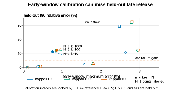
The early-window comparator supplies a second warning. A scalar diffusivity fitted only where the resolved release fraction satisfies meets the early error gate yet misses held-out by more than in exactly three declared witnesses: . Their early maximum errors are , , and , while their held-out errors are , , and .
These findings are numerical evidence for one fixed family. They are not a theorem about homogenization, not a general connectivity map, not a calibrated pharmaceutical model, and not a claim about swelling, erosion, degradation, binding, dissolution, reaction, moving interfaces, non-Fickian transport, clinical response, dose, efficacy, or safety. The literature review led to a REFRAME decision because periodic homogenization, microstructure-resolved release, connectivity effects, apparent diffusivity, and finite-transient deviations are all established. That decision makes the useful contribution a controlled finite-scale benchmark, not a new effective-diffusivity formula.
What the benchmark found
| Question | Finding | Why it matters |
|---|---|---|
| What was tested? | One 1-D periodic slow–fast–slow laminate with perfect sinks | The result concerns one transverse barrier family and one boundary phase. |
| How broad was the comparison? | and | The 24 cases include six homogeneous controls and 18 heterogeneous cases. |
| When was the harmonic model adequate? | 7 adequate, 2 grey, 9 breakdown among the heterogeneous cases | Scale separation, not the coefficient alone, controls the finite transient. |
| Where did the pattern change? | All contrasts were adequate at and | This is an empirical transition on the tested grid, not a universal cell-count rule. |
| Did early fitting predict the late event? | Three fits passed early but missed by more than | A close fit over did not guarantee late-time accuracy. |
| Were the discrepancies resolved numerically? | Nine scientific checks and 24 refinement checks passed | The classification differences are larger than the measured discretization changes. |
The distinction between “finite-scale boundary” and “homogenization fails” matters. The harmonic coefficient is the correct periodic coefficient for the declared 1-D cell problem. The benchmark asks whether a finite transient response is already close enough for specific trajectory and event tolerances. A breakdown label means that one comparator crossed one frozen numerical gate. It does not invalidate homogenization theory.
Why the literature changed the question
Heterogeneous polymer release and effective transport are not new combinations. Chandrasekaran and Hillman modeled release from a heterogeneous polymeric matrix in 1980 (DOI). Auriault and Lewandowska connected periodic homogenization, an effective diffusion coefficient, and experiment while emphasizing the conditions under which a medium can be homogenized (DOI). Rim, Pinsky, and van Osdol used three-dimensional homogenization to calculate effective diffusivity in the stratum corneum (DOI).
Resolved pharmaceutical microstructure is also mature prior art. Saylor and colleagues coupled evolving drug–polymer microstructure to release kinetics and examined connectivity changes (DOI). Laaksonen and colleagues constructed an explicit two-dimensional cellular-automata model for binary matrix and reservoir devices (DOI). Kimber, Kazarian, and Štěpánek combined microstructure-based tablet dissolution modeling with spectroscopic imaging and UV measurements (DOI). Barman and Bolin fitted stochastic three-dimensional models to imaged porous polymer films and evaluated diffusion observables (DOI).
Several papers constrain the interpretation of a scalar coefficient even more directly. Brandl and colleagues compared independently measured hydrogel diffusivities with release kinetics and found agreement in selected systems, so a benchmark must permit an adequate outcome rather than manufacture failure (DOI). Tabor and colleagues showed that transient effective diffusivity in finite inclusion-modified polymer systems can differ from stationary or infinite-medium predictions (DOI). Grund, Körber, and Bodmeier related apparent diffusivity and matrix-tablet release to porosity and a polymer percolation threshold (DOI). Donovan and colleagues used periodic homogenization for obstructed solute diffusion and checked it against Monte Carlo and experimental macromolecular-solution data (DOI).
The constitutive limitations are equally established. Salehi and colleagues derived a multicomponent stress–diffusion model for hydrophilic matrix release, showing why a static scalar Fickian coefficient cannot simply be transferred to swelling and composition-dependent transport (DOI). Wang and Tsai compared one- and two-diffusion-coefficient models for heterogeneous PVA hydrogels and polymer–drug conjugates (DOI). Giolando and colleagues built an open mechanistic model incorporating nonuniform drug distribution, porosity, degradation, and geometry and compared it experimentally (DOI). Graham and Klinge computed homogenized diffusion in strongly heterogeneous, enzymatically calcified hydrogels with finite elements (DOI).
Together, these 15 primary works block a broad headline. Periodic diffusion homogenization is established. Effective-diffusivity release is established. Connectivity, percolation, image-derived microstructure, transient deviations, multicomponent transport, and experimental validation are established. A one-dimensional synthetic chart cannot be advertised as a general drug–polymer discovery.
The bounded literature search did not find the exact combination of the stated symmetric 1-D cell, finite period count, contrast grid, and joint , , classification protocol. That negative search is not proof of absence. It merely leaves room for a transparent benchmark that can later be checked and extended.
The diffusion problem
The slab occupies
Its concentration obeys a diffusion-only conservation law,
The initial concentration is uniform,
and both surfaces are perfect sinks for ,
There is no source, reaction, binding, dissolution front, degradation, erosion, swelling, advection, stress coupling, or moving boundary. “Drug release” is the motivating language for the conserved scalar leaving this idealized slab; it is not a formulation-specific simulation.
The cumulative release fraction is
The synthetic event times are first crossings:
In the computation, crossings are linearly interpolated between adjacent output times. They summarize the shape of a release curve. They are not clinical endpoints and carry no pharmacokinetic or dose-response interpretation.
One symmetric cell and one boundary phase
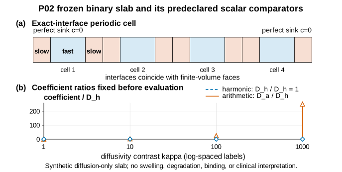
The microstructure has identical periods. In each period, the first quarter is slow, the middle half is fast, and the final quarter is slow. Thus each phase occupies one half of the slab:
The fast diffusivity is fixed at
while the slow diffusivity is
Because the unit cell is slow–fast–slow and repeats exactly, both perfect-sink boundaries meet the slow phase. That phase placement was fixed before evaluation. A different shift of the same periodic pattern could change finite- transients near the surfaces. Phase 1 does not average over shifts or perform a boundary-phase ablation.
In a one-dimensional slab, each slow layer spans the transverse cross-section. There are no paths around it. The study therefore represents connected transverse barriers, not tortuous two-dimensional routes, disconnected inclusions, random pores, or percolating three-dimensional networks.
Why the harmonic coefficient is the benchmark
For steady one-dimensional diffusion through layers in series, flux is constant across a cell. A local gradient therefore satisfies
Integrating over one cell shows that total resistance is the average of , so the periodic effective coefficient is
With equal slow and fast fractions,
This is not fitted to the release curves. It follows analytically from the frozen cell problem.
The naive arithmetic comparator is
Its ratio to the harmonic value is
That ratio is at , at , and at . In a series-layer geometry, the arithmetic mixture increasingly ignores the bottleneck imposed by the slow layers. It is included as a deliberately naive baseline, not as a serious homogenization formula for this orientation.
One nondimensional clock
All curves are reported against
The output grid is fixed at through . The horizon is not extended case by case after seeing whether an event is reached. All 24 resolved references reach both events before the fixed horizon, so none is right-censored.
For a homogeneous slab with coefficient , define . The exact perfect-sink release series is
The implementation uses 512 terms. For the harmonic comparator, . Therefore its curve in normalized time is the same for all contrasts; the resolved finite-cell curves are what change with and . For the arithmetic comparator, . For the calibrated scalar, .
The resolved microscale reference
The reference uses a conservative cell-centered finite-volume discretization. Every phase interface lies exactly on a control-volume face. The coefficient at an interior face is the harmonic face value
which is the correct series resistance for two half-cells. The canonical grid uses 256 cells and the refined grid 512. Because both counts are divisible by for every declared , the slow-quarter, fast-half, slow-quarter geometry is never blurred through a cell average.
Time evolution uses fixed-step backward Euler. The canonical run has 128 internal substeps per output interval; the refined run has 256. The symmetric implicit matrix is diagonalized once, then its eigenvalues are powered to reproduce repeated backward-Euler updates without configuration-specific step tuning.
The solver records concentration bounds, monotonicity of , a backward-Euler recurrence residual, matrix symmetry and positive off-diagonal face coefficients, and a spatial conservation check. The conservation calculation assembles face fluxes in extended precision and verifies that cell divergences telescope to the two perfect-sink outflows.
Verification before classification
No adequate, grey, or breakdown label is accepted unless the numerical checks pass.
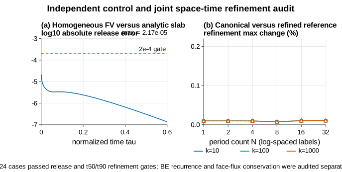
First, a homogeneous negative control compares a 1024-cell finite-volume solution with the independent analytic slab series. Its maximum absolute release error is
well below the frozen gate.
Second, every one of the 24 cases receives a joint space–time refinement. Across all cases, the largest canonical-to-refined release change is
against a limit. The largest relative change is and the largest relative change is , both far below the event-refinement limit.
Third, the recorded concentrations remain within the floating-point tolerance around . The largest saved concentration is and the smallest is positive. Release increments remain positive; the smallest recorded increment is . Maximum operator asymmetry is zero, the smallest off-diagonal coefficient is positive, the maximum mass-balance residual is , and the largest recorded backward-Euler recurrence residual is .
The nine top-level scientific checks are all true:
- homogeneous finite volume matches the analytic series;
- all cases pass joint space–time refinement;
- all concentrations stay within tolerance;
- all release curves are monotone;
- all mass-balance checks pass;
- all backward-Euler recurrence checks pass;
- all operators are symmetric with positive face couplings;
- all material interfaces are exact;
- all reference and events occur before the fixed horizon.
How the three outcomes are defined
For every heterogeneous case, the harmonic model is adequate only if
and both
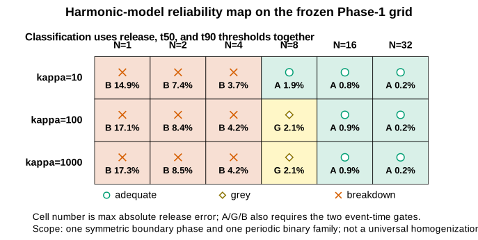
It is in breakdown if maximum release error is at least or either relative event error is at least . Any verified case between those rules is grey. The inequalities are inclusive.
This joint rule prevents a misleading classification based only on a trajectory norm. For example, at , the maximum harmonic release errors are about to , below the trajectory breakdown threshold. Yet relative errors range from to about , so all three heterogeneous cases are still breakdown cases.
The gate also permits a null outcome. If every verified case had been adequate, or none had been, the protocol would have reported that result rather than changing the grid or thresholds.
The 18-case harmonic reliability map
The exact classification is:
| Contrast | ||||||
|---|---|---|---|---|---|---|
| breakdown | breakdown | breakdown | adequate | adequate | adequate | |
| breakdown | breakdown | breakdown | grey | adequate | adequate | |
| breakdown | breakdown | breakdown | grey | adequate | adequate |
At , maximum harmonic release error falls from at to , , , , and as doubles. At , the corresponding , , and values are , , and . At , they are , , and .
The contrast dependence is exactly where the grey category earns its place. For , maximum error , error , and error all satisfy the adequate rule. At , maximum error is : just above the adequate trajectory threshold but far below breakdown, while the event errors are and . At , maximum error is and event errors are and . Both are therefore grey, not breakdown.
At , all three contrasts are adequate. Even the case has maximum release error , relative error , and relative error . At , all three remain adequate, with maximum errors near .
This grid empirically supports the first hypothesis: at each frozen contrast, harmonic accuracy improves as more periods fit into the same slab. It does not prove a convergence rate or give an error bound beyond the sampled values.
Reading two representative release curves
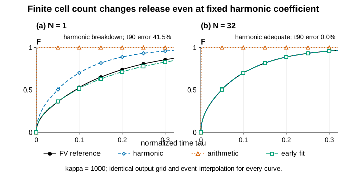
At and , the resolved reference reaches normalized and . The harmonic homogeneous curve reaches the same thresholds at and , producing relative errors of and . Its maximum release-fraction error is . This is a clear breakdown case.
At the same contrast but , the fine-period resolved curve nearly overlays the harmonic curve and the case is adequate. The coefficient has not changed: . What changes is scale separation. Thirty-two repeated cells distribute the same slow and fast fractions much more finely across the slab, so the finite transient resembles the homogenized limit.
The arithmetic curve behaves very differently because at this contrast. In normalized time it releases almost immediately and is in breakdown across the non-control grid. That result confirms the expected importance of series resistance in this geometry; it is not evidence that arithmetic averaging is always wrong in every orientation or morphology.
The early-window fit and its held-out test
The calibrated comparator chooses a scalar within
by minimizing mean squared release error only at resolved samples satisfying
The search is performed in log diffusivity with 96 fixed golden-section iterations. Samples with and the entire event are held out from fitting and tuning. As a separation check, changing only the held-out portion while keeping the early window fixed leaves the fitted coefficient unchanged.
The early-fit/late-failure gate requires an early-window maximum error no greater than and a held-out relative error at least . Exactly three cases pass both sides:
| Witness | Early max error | Held-out max error | Held-out error | |
|---|---|---|---|---|
These witnesses show a specific form of non-identifiability: a homogeneous scalar can be tuned to look good during early release yet use a coefficient roughly half the harmonic value and still miss a late event. They do not prove that early fitting always fails. Several other cases miss the early error gate, while finer cases fit early and remain acceptably close late.
The fitting cost and resolved calibration data are not free. is an empirical comparator, not an a-priori homogenized coefficient and not a deployable parameter-estimation result.
What this result shows and what remains open
The strongest supported statement is conditional:
For this fixed diffusion-only periodic slab, harmonic-model agreement improves empirically with cell count, and the frozen 24-case grid contains both adequate and breakdown regimes after independent numerical verification.
The map also shows that contrast matters near the boundary. Eight cells are enough for the case to meet all adequate gates, but the two higher contrasts remain just outside the maximum-trajectory threshold and are grey. Sixteen cells are adequate for all tested contrasts.
The result does not identify a universal number of cells. Change the boundary phase, volume fraction, layer ordering, event thresholds, sink condition, reporting norm, time horizon, or dimensionality and the map may move. The study has not performed those ablations.
The early-fit result is similarly narrow. It establishes three frozen witnesses in which a curve-calibrated scalar passes the declared early window and fails held-out . It does not prove that all fitted diffusivities are untrustworthy or that is clinically meaningful.
Why mass conservation could not be skipped
The first two calculations failed their conservation check, so their provisional adequate, grey, and breakdown labels were discarded. The problem lay in how mass balance was evaluated, not in the declared cases. The corrected calculation assembles interior and boundary fluxes in extended precision and verifies that the cell divergences telescope to the two sink outflows. The model, 24-case grid, thresholds, and fit window stayed unchanged.
After that correction, two complete calculations returned the same numerical results. Independent comparisons cover the effective coefficients, exact-interface volume fraction, harmonic face flux, analytic slab series, event interpolation and censoring, matrix structure, the spectral backward-Euler update against a direct solve, separation of the held-out fit window, and inclusive classification thresholds. The earlier failure matters because a smooth-looking release curve is still unusable if its lost mass cannot be explained by boundary flux.
Why the event times add information
A whole-curve maximum and an event-time error test different features of the same trajectory. The maximum asks for the largest vertical separation in release fraction. The event error asks how far a horizontal crossing moves. Near a shallow part of the curve, a modest vertical error can shift a crossing substantially; near a steep part, the same vertical error can produce a much smaller time shift. Neither summary can replace the other.
The cases make this distinction concrete. Their maximum harmonic-curve errors are about to , below the trajectory breakdown threshold. Their relative errors begin at , so all three are still breakdown cases. Looking only at the trajectory threshold would miss the timing error that the event definition was designed to detect.
The early-fit experiment probes a different failure. It chooses a scalar coefficient from the portion of the resolved curve with , then evaluates without refitting. The three one-period witnesses therefore fail outside the information used for calibration. Their late errors cannot be repaired by saying that the early curve looked close; the held-out event was deliberately chosen to test that extrapolation.
These metrics also suggest the next useful sensitivity study. Moving the periodic pattern relative to the two sinks could change the early boundary layers without changing the infinite-period harmonic coefficient. Repeating the same curve and event analysis over several boundary phases would show whether the transition is driven mainly by bulk scale separation or by which material touches the surface.
Limitations that cannot be averaged away
One dimension. Slow layers span the cross-section. There is no path connectivity choice, tortuosity distribution, random pore network, or percolation topology. A 2-D or 3-D material can behave differently even at the same phase fractions.
One phase arrangement. Every cell is slow-quarter, fast-half, slow-quarter, and both sinks meet slow material. Boundary-phase effects are a known finite-cell risk but are intentionally not explored.
One constitutive mechanism. is static and concentration-independent. The model excludes swelling, erosion, degradation, dissolution, binding, reaction, stress coupling, moving fronts, and non-Fickian memory.
Perfect sinks. Both boundary concentrations drop to zero immediately. Finite external mass transfer, asymmetric reservoirs, surface resistance, and changing sink conditions are absent.
Synthetic time and events. , , and are nondimensional release-curve quantities. There is no mapping to exposure, efficacy, toxicity, dose, treatment schedule, or patient outcome.
Finite parameter grid. Four contrasts and six cell counts do not provide a theorem, convergence rate, or universal validity boundary. The classifications depend on the fixed and gates.
Comparator asymmetry. is analytic, is naive, and consumes resolved calibration data and optimization. They answer different questions and do not have matched setup costs.
No final evaluation. Wider geometries, boundary shifts, random or imaged structures, external calibration, and final evaluation have not been tested. Phase 1 is a controlled numerical benchmark, not a formulation recommendation.
What should be tested next
A stronger research programme could predeclare the design, then test:
- boundary-phase shifts for the same one-dimensional cell;
- unequal phase fractions and alternative layer orderings;
- an empirical or theoretical finite- error scaling study;
- two-dimensional connected versus disconnected microstructures;
- random or image-derived morphology with traceable data;
- finite mass-transfer boundary conditions;
- concentration-dependent or multicomponent constitutive models;
- swelling, degradation, erosion, binding, reaction, or moving boundaries;
- physical calibration and external experimental validation;
- a final held-out evaluation and any venue-specific claim.
Nothing in this article claims that those stages have been run. Their results cannot be inferred from the 24-case chart.
Conclusion
An effective coefficient answers a scale-limit question. A finite release experiment asks a transient, boundary-conditioned question. When those scales are well separated in this frozen slab, the two answers agree within the declared gates. When only one, two, or four coarse cells span the slab, they do not.
The study therefore does not conclude that effective diffusivity is ineffective. It identifies where the harmonic coefficient is already effective enough for one release trajectory and two event tolerances—and where it is not—while keeping numerical error below the observed discrepancy.
The early-fit witnesses add a complementary caution: good calibration on the first half of a curve does not guarantee a correct late event. That result is especially valuable because the held-out boundary was set before fitting.
The honest ending is conditional: in this one synthetic diffusion-only laminate, effective diffusivity becomes reliable as scale separation improves, while coarse finite-cell transients and early-only calibration can cross predeclared failure thresholds.
References
- S. K. Chandrasekaran and R. Hillman, “Heterogeneous model of drug release from polymeric matrix,” Journal of Pharmaceutical Sciences 69 (1980), DOI 10.1002/jps.2600691119.
- Jean-Louis Auriault and Jolanta Lewandowska, “Effective Diffusion Coefficient: From Homogenization to Experiment,” Transport in Porous Media 27 (1997), DOI 10.1023/A:1006599410942.
- Jee E. Rim, Peter M. Pinsky, and William W. van Osdol, “Using the method of homogenization to calculate the effective diffusivity of the stratum corneum,” Journal of Membrane Science 293 (2007), DOI 10.1016/j.memsci.2007.02.018.
- David M. Saylor, Chang-Soo Kim, Dinesh V. Patwardhan, and James A. Warren, “Modeling microstructure development and release kinetics in controlled drug release coatings,” Journal of Pharmaceutical Sciences 98 (2009), DOI 10.1002/jps.21416.
- Timo Johannes Laaksonen, Hannu Mikael Laaksonen, Jouni Tapio Hirvonen, and Lasse Murtomäki, “Cellular automata model for drug release from binary matrix and reservoir polymeric devices,” Biomaterials 30 (2009), DOI 10.1016/j.biomaterials.2008.12.028.
- Ferdinand Brandl, Fritz Kastner, Ruth M. Gschwind, Torsten Blunk, Jörg Tessmar, and Achim Göpferich, “Hydrogel-based drug delivery systems: comparison of drug diffusivity and release kinetics,” Journal of Controlled Release 142 (2010), DOI 10.1016/j.jconrel.2009.10.030.
- James A. Kimber, Sergei G. Kazarian, and František Štěpánek, “Microstructure-based mathematical modelling and spectroscopic imaging of tablet dissolution,” Computers & Chemical Engineering 35 (2011), DOI 10.1016/j.compchemeng.2010.07.008.
- Zbisław Tabor, Paweł Nowak, Małgorzata Krzak, and Piotr Warszyński, “Effective diffusivity in transient state,” The Journal of Chemical Physics 139 (2013), DOI 10.1063/1.4818579.
- Julia Grund, Martin Körber, and Roland Bodmeier, “Predictability of drug release from water-insoluble polymeric matrix tablets,” European Journal of Pharmaceutics and Biopharmaceutics 85 (2013), DOI 10.1016/j.ejpb.2013.08.007.
- Ali Salehi, Jin Zhao, Tim D. Cabelka, and Ronald G. Larson, “A unified multicomponent stress-diffusion model of drug release from non-biodegradable polymeric matrix tablets,” Journal of Controlled Release 224 (2016), DOI 10.1016/j.jconrel.2015.12.045.
- Preston Donovan, Yasaman Chehreghanianzabi, Muruhan Rathinam, and Silviya Petrova Zustiak, “Homogenization Theory for the Prediction of Obstructed Solute Diffusivity in Macromolecular Solutions,” PLOS ONE 11 (2016), DOI 10.1371/journal.pone.0146093.
- Sandra Barman and David Bolin, “A three-dimensional statistical model for imaged microstructures of porous polymer films,” Journal of Microscopy 269 (2018), DOI 10.1111/jmi.12623.
- T.-C. Wang and Wei-Bor Tsai, “A biphasic mathematical model for the release of polymer-drug conjugates from poly(vinyl alcohol) hydrogels,” Journal of the Taiwan Institute of Chemical Engineers 135 (2022), DOI 10.1016/j.jtice.2022.104395.
- Patrick A. Giolando and colleagues, “Mechanistic Computational Modeling of Implantable, Bioresorbable Drug Release Systems,” Advanced Materials 35 (2023), DOI 10.1002/adma.202301698.
- Marc Graham and Sandra Klinge, “Multiscale homogenisation of diffusion in enzymatically-calcified hydrogels,” Journal of the Mechanical Behavior of Biomedical Materials 149 (2024), DOI 10.1016/j.jmbbm.2023.106244.