
A polynomial surrogate is attractive because it turns repeated nonlinear model solves into inexpensive algebra. But what happens when the model response does not merely curve, and instead jumps from one stable branch to another? A single smooth polynomial must then represent two smooth pieces and the discontinuity between them. Increasing its degree can sharpen the transition, but it can also spread oscillatory error away from the jump, move a threshold crossing, and assign mass to physically inadmissible response values.
This project tests that failure mode on one deliberately small, synthetic benchmark: a dimensionless non-isothermal continuous stirred-tank reactor (CSTR) with a saddle-node fold. The uncertain Damköhler number is centered exactly on the analytic ignition fold. A global degree-15 Legendre collocation surrogate and a two-element degree-7-plus-degree-7 surrogate each receive exactly 16 forward evaluations. The second construction places its element boundary at the known fold.
That last sentence is both the reason for the strong numerical result and its most important limitation. The fold is supplied by an analytic oracle. Its derivation and discovery cost are excluded from the matched 16-evaluation fit budget. The local construction is therefore fold-aligned, not adaptive. This is not a total-cost comparison, not a claim that an automatic algorithm found the discontinuity, and not evidence of universal superiority.
Within that narrow boundary, the Phase-1 outcome is clear. The global surrogate has response RMSE and Wasserstein-1 error . The fold-aligned surrogate has RMSE and Wasserstein-1 error . Those are improvement factors of about and . Under the declared cold-start, quasi-static, right-continuous history, the analytic hot-state probability is ; the global surrogate gives , while the fold-aligned surrogate gives . The global surrogate also places probability mass outside the valid response support, whereas the fold-aligned surrogate places none.
Those numbers belong to one fixed benchmark. They do not establish an adaptive multi-element method, a cheaper end-to-end workflow, physical reactor fidelity, industrial safety, finite-rate ignition behavior, or a theorem about polynomial chaos. The literature review led to REFRAME because polynomial chaos near bifurcations, multi-element partitioning, discontinuity detection, and uncertain CSTR analysis are established research areas. That label means testing a precise matched-fit question rather than claiming to invent multi-element polynomial chaos.
What happened near the fold
| Question | Finding | Why it matters |
|---|---|---|
| What model was used? | A synthetic dimensionless CSTR | It is a canonical numerical model, not a calibrated reactor. |
| How was branch history defined? | Cold start, quasi-static increasing , right-continuous at ignition | The response is deterministic under one history, not a finite-rate simulation. |
| What uncertainty was applied? | , | The input law is symmetric and centered on the ignition fold. |
| How were the 16 calls allocated globally? | One degree-15 fit over the whole interval | A continuous polynomial must cross the response jump. |
| How were the 16 calls allocated locally? | Two degree-7 fits, 8 calls on each side | The oracle split lets each polynomial see only one smooth branch. |
| What did the comparison establish? | All 16 scientific checks passed; status SUPPORTED | The result supports this smoke comparison, not a universal method ranking. |
| What cost was omitted? | Analytic fold location | Fit-call budgets match, but total setup costs do not. |
This separation matters because “same budget” has several meanings. The two fits use the same number of calls to the response model. Only one fit is told where to split. If locating a fold required continuation, additional solves, adjoints, experiments, or a classifier, those costs would belong in a total-cost study. Phase 1 intentionally does not estimate them.
Why the literature changed the question
The initial project title suggested a broad claim: adaptive multi-element polynomial chaos could rescue uncertainty propagation across thermal bistability in a CSTR. The literature review made that headline indefensible before computation began.
Wan and Karniadakis introduced an adaptive multi-element generalized polynomial chaos method for stochastic differential equations in 2005, explicitly establishing random-space decomposition as a response to loss of global spectral regularity (DOI). Venturi, Wan, and Karniadakis coupled polynomial-chaos ideas with stochastic bifurcation analysis for Rayleigh–Bénard convection in 2010 (DOI). Kuehn and Lux later treated uncertainty quantification of bifurcations in random ordinary differential equations with a systematic dynamical-systems perspective (DOI).
The overlap is even closer in recent work. Dréau, Magnain, and Batailly developed multi-element polynomial chaos based on automatic discontinuity detection for nonlinear systems (DOI). Kuehn, Piazzola, and Ullmann analyzed bifurcations of the Allen–Cahn equation with random coefficients (DOI). Gonnella, Khamlich, Pichi, and Rozza studied a stochastic perturbation approach to nonlinear bifurcating problems (DOI); Venier, Gonnella, Pichi, and Rozza addressed consistency and convergence of polynomial-chaos branch approximations in stochastic bifurcation analysis (arXiv DOI).
There are also two adjacent lines of work that constrain the novelty claim. Bourgey, Gobet, and Rey compared polynomial-type chaos expansions for indicator functions, directly relevant whenever a smooth surrogate is converted into an event probability (DOI). CSTRs under uncertainty are not untouched territory: Ratto and Paladino analyzed controlled CSTR models with fluctuating and uncertain parameters in 2000 (DOI), while Du, Budman, and Duever used polynomial-chaos-based Markov models in probabilistic robust self-tuning control (DOI).
These ten primary works establish the broad landscape. Global polynomial approximation can struggle when a response loses smoothness. Partitioning random space is established. Adaptive or automatic discontinuity localization is established. Polynomial chaos has been combined with bifurcation analysis, and probabilistic methods have been applied to uncertain CSTRs. A local experiment cannot honestly be presented as discovering any of those facts.
The reframed question is narrower and fully specified:
Under one frozen, fold-centered uncertainty law and one declared branch history, how different are a global polynomial and an oracle fold-aligned two-element polynomial when both fits spend 16 forward evaluations?
That question leaves a useful paper seed because it makes the comparison fully inspectable. It specifies the branch operator, the event definition, the fit budget, the oracle disclosure, the reference construction, and the pass/fail rule. The literature search supports the decision to narrow the question; it does not prove that no similar benchmark has ever existed, and the local smoke result does not overturn the established literature.
The canonical CSTR model
The dimensionless state consists of reactant concentration and temperature rise . With activation parameter , heat-release parameter , and Damköhler number , the model is
Phase 1 freezes and . These are dimensionless benchmark values. There is no mapping to a particular reaction, vessel volume, cooling system, residence time, feed composition, or industrial operating envelope.
At equilibrium, add times the concentration equation to the temperature equation. The nonlinear reaction terms cancel, leaving
so every positive steady state satisfies
Substituting this relation into either steady equation parameterizes the entire positive equilibrium curve by :
There is an important typographic point in the previous display: the expression is a product, not a sum. Written unambiguously,
The explicit multiplication symbol is included to prevent the line break from being misread; the implemented formula is .
Rather than trusting a nonlinear time integrator to reveal steady branches, the benchmark works directly with this exact scalar curve. That choice makes the branch reference and fold calculation independent of step-size or transient stopping rules.
Deriving the two folds
A fold is a stationary point of . It is numerically cleaner to differentiate its logarithm:
Setting this derivative to zero and clearing denominators gives the quadratic
For and , its two roots in produce two simple folds. The lower-temperature turning point is the ignition fold:
The higher-temperature turning point is the extinction fold:
The apparently reversed ordering of the values is exactly what produces the S-shaped equilibrium curve. Between and , three equilibria coexist: a stable cold branch, an unstable middle saddle branch, and a stable hot branch. The Phase-1 code verifies stability with the Jacobian eigenvalues rather than assigning branch labels from temperature alone.
The analytic fold values were cross-checked by an independent scan for sign changes of the logarithmic derivative followed by bisection. The absolute differences were for ignition and for extinction. The absolute temperature differences were and . Fold derivative residuals were and , and the finite-difference second derivatives had nonzero signs, confirming two simple folds under the frozen tolerances.
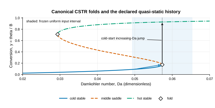
History is part of the response definition
An S-curve does not define a unique response in the bistable interval. At one , both cold and hot stable equilibria may exist. Asking a root solver for “the equilibrium” without declaring a branch rule is therefore incomplete.
Phase 1 declares an idealized history:
- Start at .
- Increase quasi-statically.
- Follow the stable cold branch for .
- At the ignition fold, take the hot branch; the convention is right-continuous.
The initial value is below the extinction value . Direct branch enumeration finds exactly one equilibrium there, and it is stable and cold. That check prevents an ambiguous starting branch from being silently built into the result.
Define the conversion-like response
Under the declared history,
The cold one-sided limit at the fold is , while the right-continuous hot value is . The jump is not numerical noise; it is the chosen history operator acting on a bistable equilibrium diagram.
This is not a dynamic ramp. The code does not integrate a finite-rate increase in , model delayed loss of stability, inject thermal noise, or calculate a random branch occupancy. Consequently, the “hot probability” below is a history-conditioned probability induced by uncertain . It is not a stationary probability of occupying the hot state and not a safety probability for a physical reactor.
The fold-centered uncertainty law
The uncertain input is
Thus the sampled interval is
with the ignition fold exactly at . A state is called hot when . Because the declared response is cold for and jumps to a hot value above for , symmetry gives the analytic protocol probability
This exact provides a particularly transparent event check. It is not a difficult probability calculation, and it should not be sold as one. Its purpose is to expose whether a surrogate shifts or smears a sharp branch transition enough to change an event measure.
The global construction
For , Legendre polynomials are a natural orthogonal basis. The global surrogate takes the form
Sixteen Gauss-Legendre nodes provide the 16 forward evaluations and the quadrature projection for the degree-15 coefficients. The code checks that the Gauss weights sum to two, that the discrete Legendre inner products satisfy the expected orthogonality, and that the fitted polynomial reconstructs its collocation nodes. The largest node reconstruction error is .
That is important: the global result does not fail because the linear algebra is visibly broken. It accurately interpolates or projects the values it was given at the collocation nodes. Its difficulty is representational. A continuous polynomial is being asked to approximate a discontinuous history-conditioned response across the whole interval.
The global approximation therefore oscillates near the jump. Its surrogate threshold occurs at , about above the true right-continuous transition. That shift turns directly into event-probability error under a uniform input.
The oracle fold-aligned construction
The local surrogate splits the physical input interval at the known analytic ignition fold:
On each element it fits a degree-7 Legendre expansion using eight Gauss-Legendre evaluations:
Here and map their respective physical elements to . The response within either branch is smooth, so each polynomial only has to approximate one smooth piece. The element boundary carries the discontinuity instead of asking a global basis to synthesize it through oscillation.
The left and right collocation-node reconstruction errors are and . The total count is response evaluations, matching the global fit.
However, the split is not discovered from those values. It is supplied by the analytic fold calculation. Calling this method “adaptive” would falsely attribute an unperformed detection step to the algorithm. Likewise, “same computational cost” would be too broad. Only the counted forward evaluations used to fit the surrogates are matched. The analytic-oracle setup cost is explicitly outside the budget.
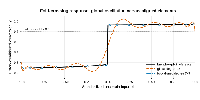
Building an independent reference
The reference response does not come from either surrogate. For each evaluation input, the named branch is solved by deterministic bisection on the exact scalar steady curve. Branch intervals are explicit: cold roots lie below the ignition temperature, middle roots between the fold temperatures, and hot roots above the extinction temperature. This prevents Newton iteration from converging to whichever nearby root happens to attract it.
The fine reference uses 32,768 midpoint cells; the coarse check uses 16,384. Moving from coarse to fine changes the global RMSE by and the global Wasserstein-1 error by . The corresponding fold-aligned changes are and . Every change is below the frozen reference-convergence tolerance.
Across sampled outer branches, the largest real eigenvalue is , remaining negative. A representative middle-branch Jacobian determinant is , consistent with a saddle. The maximum saved steady-state residual is , below the gate. These diagnostics do not validate reactor physics; they verify that the numerical reference implements the declared mathematical branches.
What the matched-fit comparison found
The core metric table is:
| Metric | Global degree 15 | Fold-aligned degree 7+7 |
|---|---|---|
| Fit forward evaluations | 16 | 16 |
| RMSE | ||
| Wasserstein-1 error | ||
| Saved absolute mean error | ||
| Hot-state probability | ||
| Absolute hot-probability error | ||
| Branch classification error rate | ||
| Invalid-support mass | ||
| One-sided fold maximum error |
The RMSE ratio is
and the Wasserstein ratio is
These large factors are not mysterious. The experimental design gives the local method exactly the structural information that the global method lacks: the location of the jump. The fair conclusion is conditional—given the analytic fold boundary, at the same fit-evaluation count, the fold-aligned representation is much more faithful on this case. It would be unfair to convert that into “multi-element PCE is always 315 times better” or “the local method is 315 times cheaper.”
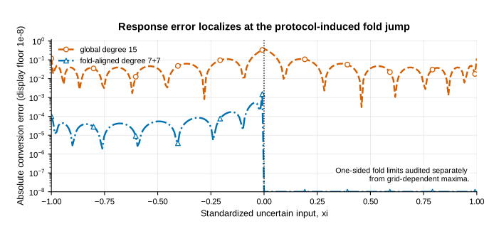
Why RMSE can be large while the absolute difference of means is small
A discontinuity concentrates very large pointwise errors in a narrow region. Squaring those errors makes RMSE sensitive to the oscillatory jump neighborhood. The other reported average is the absolute difference between the predicted and reference sample means—not the mean of pointwise absolute errors—so positive and negative oscillations can cancel before the absolute value is taken. It is therefore described as an absolute mean difference and is not interpreted as MAE.
The global absolute mean error of is not an argument that the event error is negligible. Its threshold shift produces a absolute probability error, and of the surrogate distribution falls outside valid support. Wasserstein-1 asks whether the surrogate reproduces the response distribution; the hot probability tests a declared event; invalid-support mass checks whether the polynomial invents values outside the conversion range. This is exactly why a reliability benchmark needs several metrics rather than one average.
Why the exact fold point needs special handling
The response is right-continuous and discontinuous at the fold. A dense grid usually samples close to, but not exactly at, the jump. Its maximum error therefore depends on the closest sample distance. Refining the grid can change that maximum without changing the underlying surrogate.
For this reason, the decision rule does not use dense-grid maximum error as a pass/fail criterion. The measured values are globally and locally, while the one-sided fold maximum is treated as the more stable diagnostic. This is a small but important example of designing a metric around the mathematics rather than selecting whichever number looks most impressive.
Event and support behavior
The analytic history-conditioned hot probability is . The global polynomial crosses too late, giving . The fold-aligned representation uses the declared right element at the split and gives exactly under the implemented threshold calculation.
The global polynomial also overshoots the response support . The measured input mass mapping to invalid values is . The fold-aligned surrogate has zero measured invalid-support mass on the evaluation grid. Again, that zero belongs to this one configuration; it is not a theorem that local polynomials preserve support.
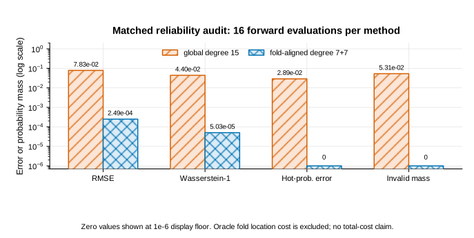
How the comparison was judged
The thresholds were chosen before interpreting the final metrics:
- at least RMSE reduction;
- at least Wasserstein-1 reduction;
- fold-aligned hot-probability error no greater than ;
- zero fold-aligned invalid-support mass on the evaluation grid;
- reference, residual, quadrature, reconstruction, fold, and stability calculations all within their stated tolerances.
The observed factors and exceed the first two thresholds. The hot-probability error and invalid-support mass are both zero, while the supporting calculations remain within their stated tolerances. The comparison therefore meets every criterion declared for this one fold-centered CSTR smoke benchmark.
Those criteria concern this comparison only. They do not rank all multi-element methods or turn a matched-fit result into a total-cost result.
Why the numerical result is credible
The analytic fold locations agree with an independent scan and bisection, their derivative residuals satisfy tolerance, and both folds are simple. The frozen initial state has a unique stable cold equilibrium; sampled outer branches remain stable, the middle branch is a saddle, and the steady-state residuals stay within tolerance. These checks support the branch history used to define the discontinuous response.
The two surrogate constructions are checked on a separate numerical layer. Gauss weights and discrete Legendre orthogonality behave as expected, collocation nodes are reconstructed to roundoff, the reference-grid refinement changes every reported error by less than , and both fits use 16 forward evaluations. Repeating the full calculation returns the same scientific metrics. This agreement supports the finite comparison without turning an oracle-aligned benchmark into an automatic or total-cost result.
How a threshold shift becomes probability error
The global surrogate’s hot-state error can be checked without treating it as a black-box statistic. The right-continuous reference changes branch at
while the global polynomial crosses at
The shift is therefore
The uniform input interval has width . Moving the left edge of the hot region to the right by removes the probability mass
That value matches the recorded global hot-probability error . The estimate is therefore understandable as , not as an unexplained quadrature discrepancy. A response error concentrated near one jump can still move several percentage points of event probability.
The fold-aligned construction does not ask one polynomial to cross that jump. Its element boundary carries the discontinuity, and the right-continuous rule assigns the fold point to the hot element. That is why it recovers in this symmetric case. The exact match still depends on oracle alignment. If the supplied split moved by , the leading probability penalty would be about until ordinary polynomial crossing errors became comparable.
This relation suggests a direct next experiment: displace the split by a declared sequence of positive and negative offsets while holding all 16 fit calls fixed. Plot event error against , then check where response approximation error causes the observed curve to depart from that simple line. Such a test would measure sensitivity to imperfect fold localization without pretending that an automatic detector has already been built.
To keep that sensitivity study interpretable, the offset grid should be fixed before its outcomes are inspected. Pilot offsets can be used to choose a useful range, while separate held-out positive and negative offsets test the final rule. Reporting the signed probability shift together with RMSE, Wasserstein error, invalid-support mass, and whether a displaced split crosses a collocation node would help separate locator bias from ordinary polynomial-fit error.
What Phase 1 does not establish
The limitations are structural, not ceremonial.
First, fold knowledge is privileged information. The analytic split is supplied before the local fit, and its setup cost is excluded. An adaptive algorithm would have to infer where regularity is lost, decide whether to split, allocate samples, and possibly revise the partition. None of those operations was implemented.
Second, equal fit calls do not imply equal total cost. Algebraic fold derivation is inexpensive here because the canonical steady curve is explicit. In a large simulator, locating a bifurcation might be comparable to—or more expensive than—the surrogate fit. The correct accounting unit for that future experiment would include continuation, diagnostics, failed searches, and any pilot evaluations.
Third, the experiment freezes one polynomial order and one budget. Degree 15 versus degree 7+7 at 16 calls does not describe convergence across orders. It does not show where the global method becomes acceptable, whether another global basis performs better, or how a local method behaves with a misplaced split.
Fourth, the input law is symmetric and centered on the ignition fold. That makes the reference event probability exactly . Off-center, skewed, correlated, or multi-parameter uncertainty could change both approximation and event behavior. No such sweep has been run.
Fifth, branch history is idealized. The response assumes a cold start and infinitely slow monotone increase, then imposes right continuity. A finite-rate system can exhibit delay and dependence on initial transients; a noisy system can switch before a deterministic fold. Those phenomena are absent.
Sixth, the model is dimensionless and synthetic. There is no data calibration, parameter-identification uncertainty, heat-transfer design, material constraint, controller, hazard analysis, or chemical safety case. “Hot” is merely the declared numerical condition .
Seventh, the decision metrics are empirical on fixed evaluation sets. Zero measured invalid-support mass is not an analytic positivity certificate. An exact event match at is not general probability accuracy. Large improvement factors on one discontinuity are not universal superiority.
Finally, the literature review is not proof that no similar work exists. It justifies the cautious local claim, but it cannot certify novelty by itself.
What should be tested next
The next experiments should address several questions:
- repeat the comparison across wider uncertainty widths, offsets from the fold, and polynomial budgets;
- perturb the supplied split to measure sensitivity to localization error;
- implement a genuinely adaptive or automatic element-discovery rule;
- charge pilot, fold-location, continuation, and failed-attempt costs;
- introduce multiple uncertain parameters and nonuniform input laws;
- compare finite-rate dynamics with the quasi-static history operator;
- calibrate a physical model only if traceable experimental evidence becomes available;
- perform a final evaluation only after its protocol is frozen;
- separate this preliminary fit comparison from any later method-level conclusion.
Listing these steps does not claim they have begun. They remain future work. In particular, there is no automatic split, no total-cost result, no calibrated physical reactor, no safety conclusion, and no final sweep hidden behind the Phase-1 figures.
Conclusion
Several conclusions do survive careful qualification.
The canonical model has two independently cross-checked simple folds. The frozen initial point lies in a unique stable cold regime. The branch-explicit reference implements the declared right-continuous history and satisfies residual, stability, and grid-convergence checks.
At a matched fit budget of 16 forward evaluations, a degree-15 global Legendre polynomial has difficulty representing the discontinuous response. It shows large RMSE and distributional error, moves the hot threshold, misclassifies part of the input domain, and assigns nonzero probability mass outside the valid response range.
When the exact ignition fold is provided as an oracle element boundary, two degree-7 expansions represent the smooth one-sided branches accurately. On this frozen case they reduce RMSE and Wasserstein-1 error by factors of about and , match the analytic history-conditioned hot probability, and show zero measured invalid-support mass.
The strongest lesson is not that local polynomial chaos “wins.” It is that a budget comparison must say what structural information each method receives and what costs are counted. Here, knowing where the response jumps is enormously valuable. Phase 1 measures that value under an intentionally favorable oracle construction. The next scientific question is how much of that value survives when the fold must be found, its cost is charged, and its location is imperfect.
Until those stages are run, the honest headline remains conditional: when polynomial chaos crosses this fold, a global polynomial is unreliable; an oracle fold-aligned representation repairs the frozen fit, but the oracle is part of the answer.
References
- Isabella Carla Gonnella, Moaad Khamlich, Federico Pichi, and Gianluigi Rozza, “A Stochastic Perturbation Approach to Nonlinear Bifurcating Problems,” Journal of Scientific Computing (2026), DOI 10.1007/s10915-026-03338-0.
- Giacomo Venier, Isabella Carla Gonnella, Federico Pichi, and Gianluigi Rozza, “Stochastic bifurcation analysis via polynomial chaos: consistency and convergence of branch-approximating solutions” (2026), arXiv DOI 10.48550/arXiv.2605.31288.
- Juliette Dréau, Benoit Magnain, and Alain Batailly, “Multi-element polynomial chaos expansion based on automatic discontinuity detection for nonlinear systems,” Journal of Sound and Vibration 567 (2023), DOI 10.1016/j.jsv.2023.117920.
- Christian Kuehn, Chiara Piazzola, and Elisabeth Ullmann, “Uncertainty quantification analysis of bifurcations of the Allen–Cahn equation with random coefficients,” Physica D 470 (2024), DOI 10.1016/j.physd.2024.134390.
- Daniele Venturi, Xiaoliang Wan, and George Em Karniadakis, “Stochastic bifurcation analysis of Rayleigh–Bénard convection,” Journal of Fluid Mechanics 650 (2010), DOI 10.1017/S0022112009993685.
- Xiaoliang Wan and George Em Karniadakis, “An adaptive multi-element generalized polynomial chaos method for stochastic differential equations,” Journal of Computational Physics 209 (2005), DOI 10.1016/j.jcp.2005.03.023.
- Christian Kuehn and Kerstin Lux, “Uncertainty Quantification of Bifurcations in Random Ordinary Differential Equations,” SIAM Journal on Applied Dynamical Systems 20 (2021), DOI 10.1137/21M1392073.
- Florian Bourgey, Emmanuel Gobet, and Clément Rey, “A Comparative Study of Polynomial-Type Chaos Expansions for Indicator Functions,” SIAM/ASA Journal on Uncertainty Quantification 10 (2022), DOI 10.1137/21M1413146.
- Yuncheng Du, Hector Budman, and Thomas Duever, “Robust Self-Tuning Control Design under Probabilistic Uncertainty using Polynomial Chaos Expansion-based Markov Models,” IFAC-PapersOnLine 51 (2018), DOI 10.1016/j.ifacol.2018.09.273.
- M. Ratto and O. Paladino, “Analysis of controlled CSTR models with fluctuating parameters and uncertain parameters,” Chemical Engineering Journal 79 (2000), DOI 10.1016/S1385-8947(00)00139-X.