How Many Equilibria Did the Optimizer Miss?

Imagine compressing a thin strip until it folds. A numerical optimizer returns an elegant shape; another initial guess returns its mirror image. After enough repetitions, the picture begins to look convincing. If all successful runs lead to the same pair of shapes, have we found everything that matters?

There are at least three different questions hidden inside that sentence. Have we found the lowest energy? Have we found every stable local configuration? Have we found the unstable equilibria separating those configurations? A method can answer the first two successfully while being deliberately unsuited to the third. Conversely, a root solver can produce many additional shapes without producing a single additional stable state.

Two pairs of minima describe a different landscape from one pair, even if the deeper pair remains unchanged. The extra pair can be metastable: locally resistant to perturbations but not globally preferred. Experimental access additionally depends on loading, forcing and dissipation, which static minimization does not determine.

The study here revisits a reduced folding energy rather than inventing a new continuation method. Deflation, pseudo-arclength continuation and solution-landscape searches already have substantial mathematical and mechanical precedents [1–8]. The useful question is narrower: what does a particular optimizer-only description retain, and what does a branch-aware description add after the roots, classifications and discretization have been checked?

The initial comparison supplied a useful negative result. On 73 loads between 42 and 60, independent multistart minimization recovered every stable reference state in both tested nonlinear parameterizations. Continuation recovered some stationary states missing from optimizer outputs, but an additional deflation stage discovered no new accepted root. Those facts did not justify saying that the optimizer had missed stable folding configurations.

A two-mode calculation then identified a more informative question beyond that original window. In one parameterization, a second pair of minima appears at a higher load, accompanied by mixed-mode saddles. In the other, it does not appear over the extended window. Small shifts in the heterogeneous loading pattern further change this secondary event. This creates a controlled test of metastability and discovery, not a reason to discard the earlier negative result.

The extension compares two nonlinear settings, two mode counts and four load phases: sixteen settings, each on 193 load slices from 42 to 90. Every tested workflow recovers all stable reference states with the fixed main initialization. The revealing differences are instead a legacy continuation trace losing stationary coverage, small purely random initialization budgets missing minima, and additional shape modes changing whether a family is stable at all.

The project overview gives a shorter account. The earlier folding article provides the original shape-steering motivation. Its nonlinear coefficients must be kept separate from those of the smaller benchmark below.

A stationary shape is not necessarily a resting place

At a valley floor, small moves go uphill; at a pass, some go downhill; at a hilltop, many do. All three can have zero first derivative.

An equilibrium calculation begins with that first-derivative condition. If the energy is $E(q;N)$ , where $q$ describes shape and $N$ describes compression, a stationary state satisfies

F(q;N)=\nabla_qE(q;N)=0,\qquad H(q;N)=\nabla_q^2E(q;N).

The Hessian $H$ supplies the local distinction. A positive-definite Hessian gives a strict local minimum. A negative eigenvalue supplies an energy-lowering direction and therefore rules out a strict minimum. The Morse index counts negative eigenvalues; an index-1 saddle has one such direction. An eigenvalue close to zero requires special care because the quadratic approximation has become weak exactly where branch structure may change.

Classification is local to the chosen shape space. Positive curvature in four coordinates does not test every continuum displacement or prescribe a specimen’s dissipative evolution.

Newton solves the zero-gradient equation, including passes and hilltops. Minimization should leave saddles, although exact symmetry or a stationary starting point can make it return one.

The flat origin is always stationary in this even energy. After its first instability it is a saddle, yet a zero starting vector can return it with a perfect residual. Software success would manufacture a false minimum if Hessian classification were omitted. Excluding it from the minimum table does not mean that the optimizer never returned it.

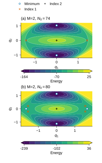
Two-mode energy contours and Hessian-classified stationary states at loads 74 and 80. — Figure 1. Zero-phase two-mode energy landscapes for the small benchmark, C=4 and S=1, at loads 74 and 80. Coordinates are shape coefficients, not measured beam positions. The independent census supplies every signed stationary state: circles are strict minima, crosses index-1 saddles, and plus signs index-2 states. Each panel has its own energy scale. Contours show equal energy, not transition paths; numerical equilibria are not automatically physically realizable shapes.

Start with an energy whose terms can be checked

The shape is represented on the dimensionless interval $0\le x\le1$ by sine modes. The endpoints therefore have zero displacement. These coordinates prescribe a reduced admissible space; the model is not a full geometrically exact rod or a calibrated tissue simulation.

y(x)=\sum_{m=1}^{M}q_m\sin(m\pi x),\qquad E(q;N)=\int_0^1\left[ \frac{B(x)}2y_{xx}^2+\frac K2y^2+\frac C4y^4 -\frac{N(x)}2y_x^2+\frac S4y_x^4\right]dx.

The bending term penalizes curvature. The quadratic foundation term penalizes displacement. Compression lowers energy through the squared slope, while the positive quartic terms prevent that destabilizing contribution from driving energy indefinitely downward. The coefficient $C$ controls amplitude stiffening and $S$ controls slope stiffening. Their relative size changes the nonlinear landscape even when the linear onset loads remain identical.

Heterogeneity is introduced through two prescribed fields:

B(x)=B_0[1+\beta\cos(4\pi x+\phi_B)],\qquad N(x)=N[1+\eta\cos(4\pi x+\phi_N)].

The fixed values are $B_0=1$ , $K=480$ , $\beta=0.12$ and $\eta=0.18$ . Holding $\phi_B=0$ , the comparison uses $\phi_N=0,\pi/32,\pi/16,\pi/8$ : prescribed pattern shifts, not measured material disorder. The mean load $N$ is labelled $N_0$ in the figures, distinguishing it from the spatial field $N(x)$ .

The small benchmark uses $(C,S)=(4,1)$ ; the earlier shape-steering study uses $(14000,42)$ . Quartic coefficients do not enter the origin Hessian, so shared linear onset loads can conceal different finite-amplitude landscapes. The two settings are not interchangeable.

After integration the energy has the form $E=q^{\mathsf T}A(N)q/2+Q(q)/4$ , where $A$ depends affinely on load and $Q$ is homogeneous of degree four. This supplies an independent identity. Multiplying the stationary equation by $q$ gives

q^{\mathsf T}A(N)q+Q(q)=0,\qquad E(q;N)=-\frac14Q(q),\qquad q^{\mathsf T}H(q;N)q=2Q(q).

Every nonzero stationary state therefore has negative energy when the quartic form is positive. Negative energy does not distinguish a minimum from a saddle. The positive radial curvature also does not remove angular downhill directions. These identities are useful checks precisely because they expose an attractive but invalid shortcut: “the root lowers energy, so it must be stable.”

Two modes let us count rather than merely search

In two modes write $q=(x_1,x_2)$ . For brevity use $u_1,u_2$ for those two coefficients below, reserving $x$ for position along the strip. At zero phase the equilibrium equations reduce to

F_1=u_1(a+u u_1^2+w u_2^2),\qquad F_2=u_2(d+w u_1^2+v u_2^2),

where

\begin{aligned} a&=\tfrac12(\pi^4+480-N\pi^2),\\ d&=\tfrac12[0.94(16\pi^4)+480-4N\pi^2(1.09)],\\ u&=\tfrac38(C+S\pi^4),\quad v=\tfrac38(C+16S\pi^4),\quad w=\tfrac34(C+4S\pi^4). \end{aligned}

This structure gives a complete finite-dimensional control. The origin is always present. Axis roots exist when the appropriate quadratic coefficient is negative. Mixed roots are obtained by solving a two-by-two linear system for the squared amplitudes; they are real only when both squares are positive. Each feasible mixed magnitude gives four signed combinations.

Enumeration never reads optimizer outputs or supplies missing-root starting guesses. Hundreds of random starts would instead remain a search: finding no new root does not prove absence.

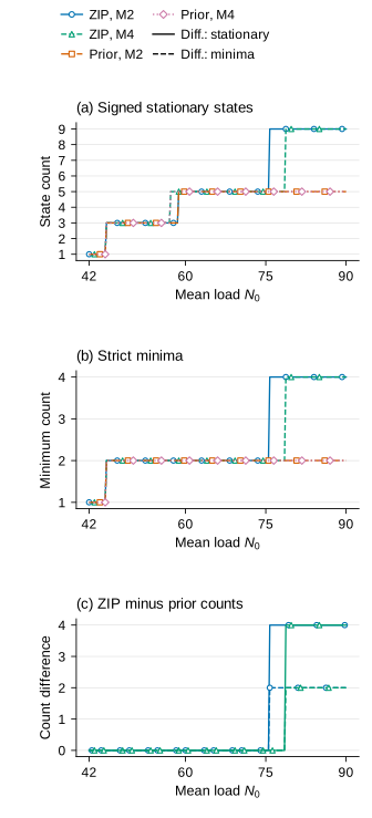
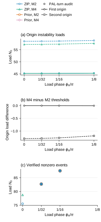
Within the first load window, the signed stationary count changes from one to three to five. The strict-minimum count changes from one to two and then stays at two. The first origin event is at approximately $45.2002335644$ and the second at $58.5037725494$ . Exactly at an event, colliding roots and a zero Hessian eigenvalue must be handled as a degenerate state, not forced into either neighboring strict classification.

The four-mode reference is a union of verified discoveries. Coverage one means recovery of that union, not every mathematical solution. Higher modes can reveal unseen families or destabilize smaller-space minima. Two-mode completeness is a method control, not a four-mode theorem.

Stationary-state and minimum counts for two nonlinear coefficient sets and two truncations. — Figure 2. Zero-phase counts on 193 loads compare the small benchmark, C=4 and S=1, with the earlier C=14000 and S=42 coefficients. Panels (a,b) separate stationary states from strict minima; panel (c) subtracts earlier-study counts from benchmark counts, exposing intentional coincidences. Solid difference curves count stationary states, dashed curves minima. Sign partners count separately. Two-mode counts have independent census certification; four-mode counts are empirical discovery unions. Connecting sampled loads does not locate intervening events or certify complete branch topology.

A larger load creates a more useful test

The zero-phase two-mode benchmark has a secondary event at $N\approx75.5468884668$ . Below it, the first-mode axis pair is saddle-like. Above it, that pair becomes locally stable and four mixed-mode index-1 saddles are present. The signed count changes from five to nine, while the strict-minimum count changes from two to four.

This is qualitatively different from adding two more unstable roots. It introduces another locally stable shape family. Yet it occurs only in the $(4,1)$ setting over the load interval considered. With the earlier $(14000,42)$ coefficients, the two-mode calculation retains five stationary states and two strict minima through load 90. A nonlinear coefficient change can therefore alter the later landscape without changing the initial linear instability.

The range ends at 90, before the next origin instability in representative higher-mode checks. This targets secondary families associated with the first two modes without ruling out other nonlinear families below 90.

Amplitude increases with load; maximum displacement and slope therefore accompany the energy results. A consistent polynomial model is not proof that a real strip remains within its mechanical assumptions or can realize every computed state.

Shift the pattern, but keep track of the remaining symmetry

Zero-phase heterogeneity preserves spatial reflection. Moving the load pattern away from zero generally breaks that reflection symmetry. It does not break the global sign symmetry: every term in the energy remains even under $q\mapsto-q$ . An upward shape and its downward sign partner still have equal energy.

For two modes the phase shift introduces a quadratic coupling. The equations become

F_1=a u_1+b u_2+u u_1^3+w u_1u_2^2,\qquad F_2=b u_1+d u_2+w u_1^2u_2+v u_2^3,

with

b=\frac{176N\eta\pi}{105}\sin\phi_N,\qquad d=\tfrac12[0.94(16\pi^4)+480-4N\pi^2(1+0.09\cos\phi_N)].

The independent control can still count all directions. When $b\ne0$ , a nonzero root cannot have $u_1=0$ . Put $t=u_2/u_1$ and eliminate the amplitude:

-bv t^4+(dw-av)t^3+(du-aw)t+bu=0,\qquad u_1^2=-\frac{a+bt}{u+wt^2}>0.

There are at most four real directions, each supplying a signed pair, in addition to the origin. A reciprocal chart uses $u_1/u_2$ for nearly vertical directions; dividing by a very small first coefficient should not make a state disappear from the count.

The calculation uses exact-rational isolation together with outward intervals for the analytic coefficients. Sturm sign variations count real polynomial roots; interval versions check that the count persists for the coefficient enclosure rather than merely for rounded midpoint coefficients. Positive squared amplitudes and Hessian classification receive their own checks. Near coalescence, uncertainty is retained instead of announcing completeness from an ill-conditioned floating root list.

Separate checks of saved pseudo-arclength turns verify two-mode folds near loads $82.6870681680$ for $\phi_N=\pi/32$ and $87.5226471200$ for $\pi/16$ . No additional two-mode stable family appears on the 193 sampled slices for $\pi/8$ within the selected window. These statements concern the declared finite model and sampling range, not events on an untested extended load interval.

The quick shared event scan missed both small-phase folds. Its near-zero-eigenvalue trigger was 5, whereas the closest sampled branch states had absolute eigenvalues of roughly 14 and 29. A coarse event trigger can therefore miss a genuine turn even when the branch itself has been saved. The supplementary verification used those saved tracks; it did not retroactively supply new seeds or change the original method coverage. Event detection and root recovery deserve separate scores.

Origin thresholds and locally verified secondary events across four load phases. — Figure 3. With stiffness phase zero, the load phase takes 0, π/32, π/16 and π/8. Panel (a) plots both origin instabilities, shared by the two nonlinear coefficient sets; panel (b) makes their M4-minus-M2 differences explicit. Panel (c) shows locally verified nonzero events: filled markers are folds, open markers reflection-symmetric secondary events. Black rings identify folds checked afterward from saved pseudo-arclength turns, without changing original seeds, costs or coverage. Sign partners form one event orbit. An absent marker does not prove an absent event.

More stable states do not necessarily change the best energy

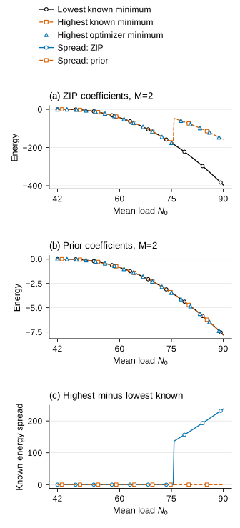
At load 80 in the zero-phase two-mode $(4,1)$ energy, the first-mode minima have energy approximately $-73.97685223$ . The second-mode minima have energy approximately $-239.18900751$ . At load 90 the corresponding values are $-158.81386915$ and $-396.40585285$ . The new family is locally stable but remains higher in energy.

A map showing only the lowest energy would therefore remain on the deeper family. A map recording every strict minimum would change. The highest-minimum curve in Figure 4 is an envelope over that changing set: it can jump when a new family enters, without any energy discontinuity along a connected branch. A transition map would additionally need saddles and paths.

Coercivity and complete two-mode enumeration permit a global energy comparison. Four- or twelve-mode discovery unions supply the lowest known energy, absent a global bound or complete enumeration.

Metastability is not a measured residence time: large disturbances can leave a local well. Waiting times require dynamical and stochastic assumptions beyond a static Hessian.

Complete two-mode controls expose a higher-energy minimum family and a negative comparison. — Figure 4. Complete zero-phase two-mode controls compare the two coefficient sets on separate energy scales. Black and orange curves bound the energies of strict minima; blue triangles show the highest-energy retained optimizer minimum. The benchmark gains a higher-energy family, while the earlier coefficients retain one sign-paired minimum energy. Panel (c) plots highest-minus-lowest minimum energy, including intentional zero differences. These are envelopes over existing minima, not individual branches: entry of a new minimum can cause a jump. Energy spreads are not transition barriers, and two-mode completeness does not establish continuum ordering.

Different workflows acquire different information

Independent multistart solves each load without previous-load information: a baseline for the pointwise atlas, not a branch-aware optimizer initialization.

Natural continuation instead carries a known stationary state to the next load. A stronger version predicts the change in shape from the tangent equation

H(q;N)\frac{dq}{dN}+F_N(q;N)=0,\qquad F_N=-Gq.

When $H$ is nonsingular, this supplies a first-order predictor before Newton correction. Near a bifurcation, the inverse becomes poorly conditioned. At a fold, load ceases to be a good local coordinate along the branch. Merely tightening Newton’s stopping rule cannot repair that geometric problem.

Pseudo-arclength treats shape and load as joint unknowns. A tangent predictor and hyperplane correction let load turn backward while arclength advances. This established numerical tool, not a new mechanical mechanism, also appears in current multiparameter work [4].

Deflation changes a root-search equation to discourage convergence to roots already found. Schematically, if $q_j$ are known states, a shifted multiplier is

\widetilde F(q)=\left[\prod_j\bigl(\|q-q_j\|^{-2}+1\bigr)\right]F(q).

Its Jacobian includes the multiplier derivative; multiplying the original Hessian by the scalar alone omits part of the Newton equation. A small deflated residual also cannot replace checking the original gradient [1]. Singular multipliers, rediscovered roots and failed attempts all need to remain visible.

These methods receive shared ordinary-root anchors and shared branch-switch candidates. The independent census is consulted only after discovery. The deflated workflow includes the earlier continuation work plus its extra attempts. Giving it more information and then calling its success an equal-cost comparison would be unfair.

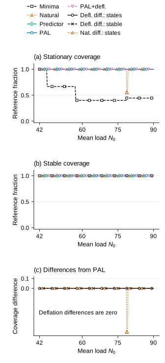
The extended comparison preserves that negative result. All five workflows recover every stable reference across all sixteen settings. Tangent-predictor natural continuation, pseudo-arclength and the deflated workflow also recover every stationary reference. Legacy previous-state natural continuation alone falls to 5/9 stationary recovery in the zero-phase four-mode small benchmark, while retaining full stable recovery. Extra deflated anchor searches accept no new roots in 16,384 attempts and add none beyond pseudo-arclength. This is evidence about a well-seeded problem, not a universal verdict: disconnected beam diagrams show discovery devices matter elsewhere [2,5].

Five methods' stationary and stable coverage against an incomplete four-mode reference. — Figure 5. The zero-phase four-mode benchmark uses the fixed 128-start bank and shared root anchors. Panel (a) compares stationary recovery against an empirical reference; panel (b) compares Hessian-verified minima. Panel (c) shows differences from pseudo-arclength: legacy natural continuation loses some stationary states, whereas adding deflation gives zero stationary or stable gain. The minimum natural recovery, 5/9, is marked explicitly. This is the only such natural-coverage loss among the sixteen settings; stable recovery is complete throughout. Slice coverage does not certify connected-branch tracking, equal budgets or higher-dimensional completeness.

Starting guesses are part of the scientific comparison

An initialization is not neutral. A coordinate-axis start in the zero-phase two-mode system lies in an invariant subspace. It can give direct access to a family that a generic random start rarely reaches. After a phase shift introduces coupling, that same vector no longer defines an invariant direction.

The main bank uses 128 fixed physical-coordinate starts: the origin, signed coordinate directions and a deterministic random remainder. Every method’s information is recorded. Smaller prefix budgets ask how recovery changes before the full bank is exhausted; expanded and additional deterministic banks test whether a conclusion depends on one favorable sample.

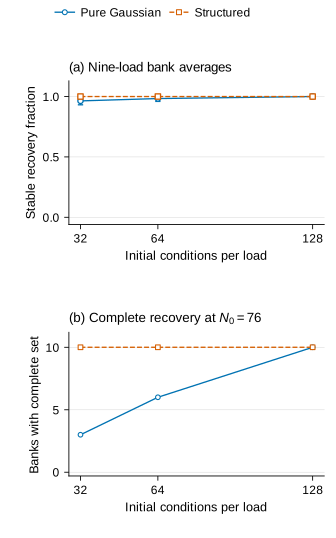
The two-mode zero-phase benchmark at load 76 makes this dependence concrete. All four strict minima are recovered in only 3 of 10 purely Gaussian banks at 32 starts. At 64 starts the count rises to 6 of 10; at 128, all 10 recover all four. Structured banks recover all four in every replicate at all three budgets. These are ten initialization replicates of one energy problem, not ten specimens or independent physical systems.

The incomplete sets differ too. At 32 starts, four banks miss the whole higher-energy sign orbit and three miss only one partner; at 64, those counts are one and three. These are two-mode omissions, not proof of a stable higher-mode family.

At load 80, the purely Gaussian recovery counts are 8/10, 9/10 and 10/10 at the same budgets. The unsuccessful banks miss one sign partner, not an entire metastable family: both symmetry orbits are represented. The higher-energy pair also corrects to strict minima in twelve modes. That is a local higher-mode re-solve, not a twelve-mode initialization experiment; the missed signed state belongs to a family that survives the stated refinement.

The frozen main bank also recovers the additional pair. Thus the statement supported here is not that multistart necessarily misses metastability. It is that a small purely random budget can omit verified minima, while a modest structural prior or a larger budget repairs that omission in this control. Reporting only the successful 128-start result would hide that difference; reporting only a failed small bank would unfairly condemn the stronger baseline.

Recovery fractions describe the initialization distribution and algorithm, not physical basin volumes. Physical attraction requires an evolution law, metric and disturbance distribution.

Software success can miss the gradient threshold; software failure can return an acceptable residual. Mathematical checks, rather than the favorable flag, determine acceptance.

Some positive-Hessian optimizer returns receive an accuracy-only root polish from that same point. This extra work is counted. An indefinite return is not polished into a minimum, and the procedure never uses the census to supply a missing starting state. The baseline is therefore minimization with a disclosed stationarity polish, not an untouched software output.

Testing metastability does not retroactively turn the original complete stable coverage into failure. Modest structured multistart can remain enough.

Paired Gaussian and structured bank recovery of the complete two-mode minimum set. — Figure 6. Ten paired initialization banks compare pure Gaussian draws with the same draws after prescribed slots are replaced by the origin and signed coordinate starts. Budgets 32, 64 and 128 are nested prefixes. Panel (a) first averages each bank's stable coverage over nine diagnostic loads, then shows the ten-bank mean ± one sample standard deviation—not a confidence interval. Panel (b) counts banks recovering all four certified minima at load 76. The observed recovery markers coincide at 128 starts; the initialization banks remain different. Lines are visual guides, not measurements of intermediate budgets or physical basin probabilities.

A correct root can still be the wrong branch

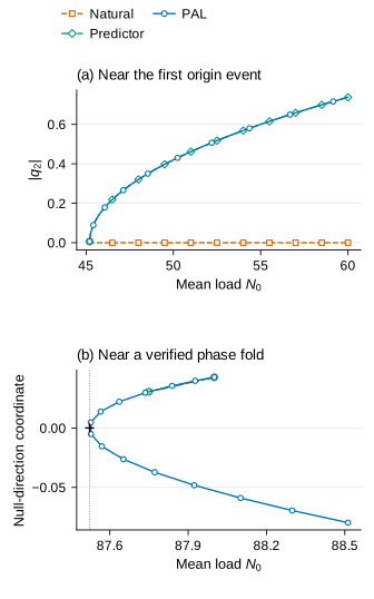
The original branch-tracking stress test starts just beyond the first instability. At four modes, the small nonzero branch is stationary, but its amplitude is close to zero. Previous-state natural correction can return to the flat root as the load increases. The flat root has zero residual, so a residual check alone cannot detect the lost branch identity.

At both tested natural steps, this occurred while pseudo-arclength preserved the nonzero branch. Yet natural continuation’s overall slice coverage was still complete because other anchors reached the missing states. “Every slice was covered” and “this trace stayed on its branch” are therefore different results.

The extension also tests tangent-predictor natural continuation: comparing pseudo-arclength only against previous-state correction would overstate its advantage. The legacy failure remains visible while the stronger predictor tests its remedy.

Secondary symmetry events need another precaution. The cubic coefficient governing a nonzero branch is not simply the positive quartic energy evaluated on a null eigenvector. Other coordinates relax as the new direction grows. Eliminating that relaxation can make the effective cubic negative even though the full quartic energy remains positive.

In the two-mode higher-load event, this reduced coefficient is $v-w^2/u<0$ . It explains why the mixed saddles appear on the side where the original axis family becomes locally stable. Reusing the origin-pitchfork formula with a positive cubic would generate starts on the wrong side. This is a mathematical issue in branch switching, not a reason to change a random seed.

For an imperfect-pattern fold, local checks include the zero-gradient equation, one null Hessian direction and nonzero load and nonlinear coefficients in that direction. Nearby accepted states provide further numerical evidence. They do not certify the absence of other roots outside that local neighborhood.

Natural, tangent-predictor and pseudo-arclength tracks near a branch birth and a verified fold. — Figure 7. Panel (a) follows the same near-origin four-mode seed with previous-state natural, tangent-predictor natural and pseudo-arclength continuation. Panel (b) uses the two-mode π/16 fold at 87.52264712, plotting matched saved tracks from 0.8 below to 1.2 above its load. The vertical coordinate projects the shape difference onto the Hessian null direction, not physical displacement. Only accepted roots are connected; failed and outside-window portions are not bridged. Natural load steps and arclength steps are different progress units. A locally preserved branch does not prove complete discovery or a physical transition.

Integration error can imitate a model change

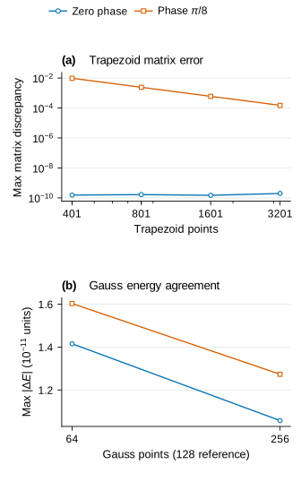
The energy contains integrals, and numerical integration is part of its realization. At zero phase, the integrands are finite cosine combinations. A sufficiently resolved uniform trapezoid rule has special exactness to roundoff in this setting. Near-identical values at 201, 401, 801 and 1601 points are therefore unsurprising.

A nonzero phase introduces sine contributions that do not inherit this particular exactness. The off-diagonal two-mode coupling is a sensitive example. At load 80 and phase $\pi/32$ , an 801-point trapezoid approximation differs from its analytic value by roughly $9.1\times10^{-5}$ . That error is small beside some diagonal entries but large compared with a $10^{-8}$ original-gradient acceptance threshold.

Near a bifurcation, a small coefficient error can also move the event or change the sign of a small Hessian eigenvalue. A beautiful, smooth branch diagram could then be a faithful solution of the wrong numerical energy. Newton convergence does not distinguish the intended integral from its approximate realization.

The phase comparison uses Gauss integration for the main energy and checks several Gauss orders independently. Trapezoid refinement is retained as a convergence experiment rather than advertised as exact. The analytic two-mode coefficients supply a further independent target.

Analytic counting, root reconstruction and compatibility with the numerical energy are separate checks. A clean surrogate root list cannot override failed compatibility with the intended model.

Zero-phase special quadrature accuracy versus nonzero-phase convergence and Gauss agreement. — Figure 8. Four-mode integration sensitivity compares zero phase with π/8. Panel (a) shows the largest linear-matrix discrepancy against Gauss-128 over the refinement loads, using 401, 801, 1601 and 3201 trapezoid points. Zero phase has special Fourier-product exactness to roundoff, not a general quadrature guarantee. Panel (b) compares accepted root energies under Gauss-64 or Gauss-256 with matched Gauss-128 corrections; the reference's tautological zero is omitted. Failed or unpaired comparisons are counted rather than assigned zero. Agreement of known roots does not enumerate unknown branches.

Adding modes changes what stability means

Four coefficients describe a richer shape than two, but neither is the continuum beam. Additional modes introduce extra directions in which a stationary state can lower its energy. A minimum in a restricted space can therefore become a saddle in a larger one even when its plotted shape changes only slightly.

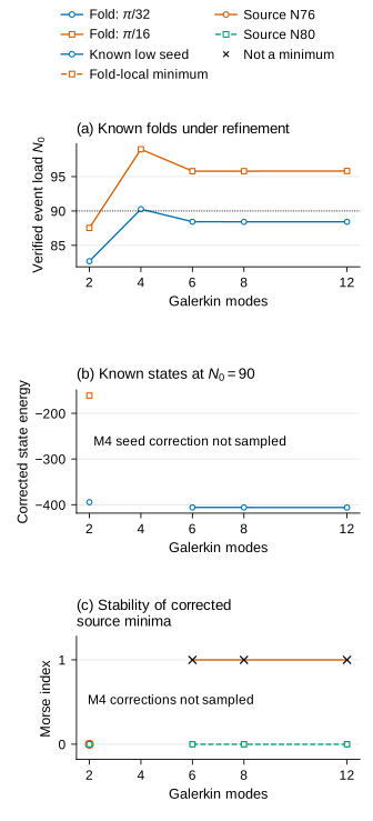
The original zero-phase refinements already show measurable changes. The first origin event moves from approximately $45.20023356$ at four modes to $45.17291168$ at twelve. The second moves from $57.20833683$ to $57.18083353$ . At load 60, the deeper $(4,1)$ minimum changes from energy $-43.26117208$ to $-44.10435142$ .

Those are not numerical integration effects: independently integrated energies agree much more closely. They come from changing the admissible shape space. A state can survive refinement while its energy and event location shift enough to matter for a quantitative claim.

The larger-load comparison includes its own refinement. Small truncation effects near onset do not bound errors at a larger amplitude. A Newton correction after padding a four-mode state with zeros checks whether a nearby higher-mode stationary state can be found. It does not enumerate every higher-mode family, and it may switch destinations if the original seed is poorly conditioned.

Here refinement changes the qualitative answer. The zero-phase secondary event moves from $75.546888$ at two modes to $78.740022$ at four and $77.992739$ at twelve. At load 76 the new two-mode pair corrects to index-1 saddles in twelve modes; at load 80 the refined pair remains minima. This is not merely a small energy correction: the admissible space changes the stability label.

Phase-shifted events are similarly sensitive. For $\pi/32$ , the verified four-mode fold is near $90.2636$ , just outside the main window, while six-, eight- and twelve-mode refinements lie near $88.42$ , inside it. For $\pi/16$ , the twelve-mode event moves to approximately $95.8055$ , outside. An event being inside or outside a plotting window can therefore depend on truncation. A four-mode discovery union alone cannot prove a family absent, and a two-mode control alone cannot establish its higher-mode stability.

Refinement retains seeds, corrected states, residuals, Morse indices, energy and geometry. Persistence requires a credible shape and low-mode association, not merely another accepted root; stability changes and failed associations remain results.

Grid-based prominent-extremum counts are descriptors, not exact counts of every analytic oscillation. Positions, amplitudes and slopes distinguish structural shifts from features near the detection threshold.

Known phase-fold shifts, π/16 endpoint energies, and a zero-phase two-mode minimum corrected to a saddle at load 76 but not 80. — Figure 9. Local Gauss-128 refinements, not a high-mode census. Panel (a) re-solves the π/32 and π/16 folds, retaining verified events beyond load 90. Panel (b) checks the π/16 lowest-known source and fold-descended minimum at load 90; outside-window folds leave the latter endpoint unattempted. Panel (c) follows positive-q1, higher-energy zero-phase two-mode minima: the load-76 source becomes index 1 at M6, M8 and M12, while load-80 corrections remain index 0. Black crosses mark accepted non-minima. Unsampled M4 source corrections are gaps; connecting stored mode counts does not locate an intervening stability boundary or prove global family identity.

Fewer solves do not automatically mean cheaper science

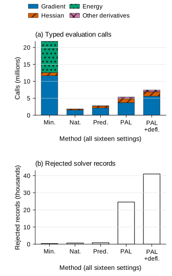
Repeated minimization pays for many energy and gradient evaluations at every load. Continuation can reuse a root and its tangent, often requiring much less work once an anchor is known. But finding anchors, scouting events, switching branches and sampling traced components also costs time.

Deflation adds more root attempts and a multiplier derivative. A workflow that finds no new state can still be scientifically useful as a robustness check, but that extra expense is not a speed improvement. Conversely, a method that solves many fewer nonlinear systems may spend more time assembling or factoring a difficult matrix.

The comparison records energy, gradient, Hessian and load-derivative evaluations, along with elapsed solver time. Shared discovery is charged to every continuation workflow that receives its information. The deflated workflow includes its earlier pseudo-arclength work. Neighbor verification and retries are retained rather than charged twice or excluded selectively. Logged solver records are accounting entries, not automatically a count of distinct nonlinear solves; a trace can contain summaries, retries and tangent evaluations.

These are transparent work summaries, not an equal-budget efficiency theorem. Different workflows solve different subproblems; branch-switch construction, eigenproblems, classification, plotting and some tensor assembly sit outside the solver totals. Wall-clock time also depends on hardware and library behavior. Repeating the full calculation reproduced its scientific summaries, with measured durations treated separately rather than required to agree.

Typed evaluations and rejected solver records with shared and composite method costs included. — Figure 10. Instrumented work sums all sixteen settings. Panel (a) separates gradient, Hessian, energy and other derivative calls; panel (b) retains rejected work records, including failed corrections and retries. Each continuation workflow pays for its shared anchors and event checks; adding deflation includes the entire pseudo-arclength cost plus extra searches. Records are not literal nonlinear-solve counts, and calls are not equal-cost operations. Branch-switch eigenproblems, assembly and editorial analyses are not exhaustively counted. The different budgets and work profiles do not establish an overall speedup.

What a saddle can tell us about a transition

An index-1 saddle is a plausible transition candidate because it has one local downhill direction. Perturbing along the two signs of that direction and minimizing can reach distinct verified minima. This checks a local energy-lowering displacement and candidate endpoints.

It does not reconstruct a continuous physical trajectory. The optimization algorithm may jump, use a nonphysical metric or follow a path that is not a minimum-energy path. A saddle energy minus a minimum energy is therefore not automatically the activation barrier governing a real transition.

A stronger study would specify dynamics or a path principle, track continuous connections, verify endpoint convergence and refine the path independently. It might also need geometry and material validation outside the reduced energy. Existing mechanical landscape studies combine several such layers [6,7]; conditional landscape theory likewise has assumptions that degenerate bifurcation points do not automatically satisfy [8,10].

Here the static audit stops short of that claim. Saddles add structure to the energy picture. Whether they control switching remains a separate question with separate evidence.

Conclusion: ask which map the computation has earned

An optimizer-only shape atlas is not inherently wrong. Over the original comparison window it recovered all stable reference states. Additional root methods filled in some unstable structure without changing that stable-state result. Preserving this negative finding is more informative than turning every new saddle into a missed minimum.

The higher-load and phase comparisons separate emerging metastable families from the deeper energy family, retain the global sign symmetry, and supply independent low-dimensional counts against which discovery can be scored. Their strongest caution is already concrete: a verified two-mode minimum can become a higher-mode saddle, and a refined event can move across the selected load boundary.

The scientific contribution is therefore the separation of questions and evidence in one specified folding model. Lowest known energy, all recovered minima, traced stationary branches and physically validated transitions are different maps. A reliable calculation tells the reader which of those maps it has earned, and which still requires another experiment.

References

Farrell, Birkisson and Funke. Deflation techniques for finding distinct solutions of nonlinear partial differential equations (2015). Primary paper.
Farrell, Beentjes and Birkisson. The computation of disconnected bifurcation diagrams (2016 preprint). Inspected preprint.
Farrell. Computing multiple solutions of systems of nonlinear equations with deflation (2026). Bibliographic record and abstract were accessible; no detailed theorem from the inaccessible full text is used here. Published record.
Kumar, Pichi and Rozza. Bifurcation curve detection with deflation for multiparametric PDEs (2026, version 2). Primary preprint.
Xia, Farrell and Castro. Nonlinear bifurcation analysis of stiffener profiles via deflation techniques (2020). Published paper.
Medina, Farrell, Bertoldi and Rycroft. Navigating the landscape of nonlinear mechanical metamaterials for advanced programmability (2020). Published paper.
Bonthron, Pierce and Tubaldi. Programming stability and stiffness in two-dimensional multistable structures (2026). Published paper.
Su, Wang, Zhang, Zhao and Zheng. Improved High-Index Saddle Dynamics for Finding Saddle Points and Solution Landscape (2025). Published paper.
Pichi and Strazzullo. Deflation-based certified greedy algorithm and adaptivity for bifurcating nonlinear PDEs (2025). Its certification concerns reduced approximations under stated conditions, not unconditional root enumeration. Published paper.
Yin, Yu and Zhang. Searching the solution landscape by generalized high-index saddle dynamics (2021). Published paper.