Steering Folds with Weak Mechanical Heterogeneity

Folding is one of the most visible ways in which growth becomes geometry. A flat sheet or slender strip accumulates compression; remaining flat becomes energetically expensive; a patterned shape appears. The classical calculation asks when buckling begins and which linear mode loses stability first. A design-oriented question goes further:

Can weak spatial heterogeneity steer the number and location of folds created by differential growth without increasing peak deformation cost?

The word “steer” matters. The experiment does not add a large geometric obstacle or prescribe the final shape. It introduces modest spatial variations in bending stiffness and compressive growth load, then asks how the equilibrium selected by a nonlinear energy changes.

This is a reduced continuum-mechanics study. It is not a calibrated model of a named tissue, organ, or manufactured laminate. Its value lies in making the mechanism, baseline, optimization, and numerical checks inspectable.

Atlas of equilibrium fold shapes under different stiffness and growth-load heterogeneity patterns. — **Figure 1.** Equilibrium shape atlas. Each curve is an energy-minimizing configuration under a declared heterogeneity; fold identity is encoded by position and line style as well as colour.

Begin with an energy, not a desired picture

Let $y(x)$ be the transverse deflection of a unit-length strip. The reduced energy is

\mathcal E[y]=\int_0^1\left[ \frac{B(x)}{2}y_{xx}^2+\frac K2y^2+\frac C4y^4 -\frac{N(x)}2y_x^2+\frac S4y_x^4 \right]\,dx.

Every term has a role.

$B(x)y_{xx}^2/2$ penalises curvature, with spatially varying bending stiffness $B(x)$ .
$Ky^2/2$ represents an elastic foundation that resists displacement.
$Cy^4/4$ prevents unbounded amplitude and supplies nonlinear saturation.
$-N(x)y_x^2/2$ is the destabilising compressive growth load.
$Sy_x^4/4$ penalises large slopes and helps regularise post-buckling shapes.

The model is phenomenological. It compresses a richer morphoelastic system into a scalar deflection and an energy landscape. That simplification is useful because it makes the competing mechanisms explicit: curvature cost, foundation cost, compression release, and nonlinear stabilisation.

The endpoint displacement conditions are built into a sine expansion,

y(x)=\sum_{m=1}^{M}q_m\sin(m\pi x).

Optimization therefore occurs over coefficients $q_m$ rather than arbitrary grid values. This does not automatically enforce every possible beam boundary condition; it enforces the declared zero-displacement endpoints exactly and provides a controlled finite-dimensional approximation.

The homogeneous linear threshold is the audit baseline

Before solving the heterogeneous nonlinear problem, set $B(x)=B$ and $N(x)=N$ , then linearise around $y=0$ . A single mode $\sin(m\pi x)$ has quadratic energy proportional to

B(m\pi)^4 + K - N(m\pi)^2.

The mode loses linear stability when

N=N_c(m)=B(m\pi)^2+\frac{K}{(m\pi)^2}.

For the declared $B=1$ and $K=480$ , mode 2 has the smallest threshold, $N_c\approx51.637$ . This analytical value does two jobs. It checks the implementation, and it provides a reference for interpreting nonlinear equilibria near the chosen load.

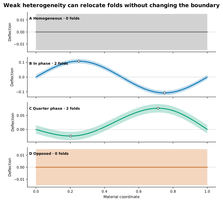
The representative nonlinear configuration uses a mean load of 48 with spatial modulation. Although 48 is below the homogeneous mode-2 threshold, heterogeneity and nonlinear energy selection can create locally favourable deformation. This is not paradoxical: the analytical number belongs to a homogeneous linearised model, while the optimization solves a heterogeneous nonlinear one.

How heterogeneity enters

The experiment uses smooth periodic modulations such as

B(x)=B_0\left[1+\beta\cos(2\pi r x+\phi_B)\right],

N(x)=N_0\left[1+\eta\cos(2\pi r x+\phi_N)\right].

Here $\beta$ and $\eta$ control amplitudes, $r$ controls the number of heterogeneity waves, and the phases decide where soft or strongly compressed regions lie.

The representative values are modest: stiffness heterogeneity $0.12$ and load heterogeneity $0.18$ , with two spatial waves. “Weak” is therefore an explicit statement about parameter amplitude inside this model, not a universal biological category.

Several initial coefficient vectors are optimized for each configuration. This is necessary because a nonconvex energy can contain multiple local minima. Reporting only one initialization would conflate “the optimizer found this state” with “this state is the unique equilibrium.”

What it means to target a fold

Fold count is estimated from the extrema of the equilibrium shape after excluding negligible numerical ripples. Location is measured relative to a target region. Mechanical cost is represented by quantities including total energy and peak absolute curvature.

These objectives can conflict. Concentrating deformation near one location may improve targeting but increase curvature. Adding more folds may distribute compression yet create an unwanted geometry. The study therefore treats the result as a Pareto-style comparison rather than reducing everything to one hidden score.

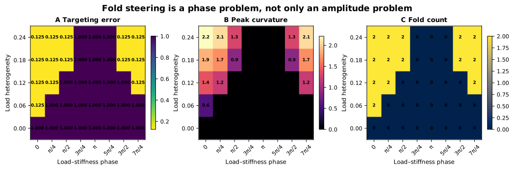
Steering map relating stiffness and load heterogeneity to fold count, location error, and peak curvature. — **Figure 2.** Steering map. Weak heterogeneity does not act as a simple on/off switch: it reshapes a multi-objective landscape of fold placement, count, and curvature.

Across the tested map, the optimizer converges in every configured case according to its numerical success and gradient criteria. The best targeting error is $0.125$ in unit-domain coordinates. The representative baseline equilibrium has two folds, energy approximately $-0.03127$ , and peak curvature approximately $1.857$ .

The important interpretation is not that $0.125$ is a biologically meaningful positional precision. It is that spatial modulation moves equilibrium features in a measurable and reproducible way while allowing curvature cost to be compared.

The map also resists an overly clean narrative. Some heterogeneities change fold position without changing count. Others cross a basin boundary and select a different number of folds. Phase can matter as much as amplitude because it controls whether a soft region aligns with a compression maximum.

Numerical optimization can lie quietly

Energy minimization is not verified merely because a library returns “success.” Three questions must be separated.

Stationarity: is the gradient small?
Discretization: does the equilibrium persist as quadrature is refined?
Globality: did multiple starts find competing minima?

The baseline gradient norm is approximately $1.27\times10^{-9}$ , supplying strong evidence of numerical stationarity in coefficient space. Quadrature refinement from 201 to 401 and 801 points produces relative shape errors of approximately $9.0\times10^{-5}$ and $2.18\times10^{-5}$ against the finest curve. Energy and fold count remain stable.

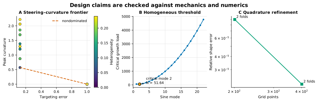
Pareto comparison and numerical verification of morphoelastic folding equilibria. — **Figure 3.** Trade-off and verification panel. Curvature, targeting, gradient norm, and grid refinement are shown together so optimizer success is not mistaken for physical validation.

These checks establish a well-resolved stationary point for the finite-mode model. They do not prove that no lower-energy state exists outside the chosen mode truncation, nor that the reduced energy is the correct constitutive model for a tissue.

Why curvature is a useful but limited cost

Peak curvature is attractive because it is geometrically clear and often related to bending strain. Yet its meaning depends on thickness, constitutive law, dimensional scaling, and whether the strip theory remains valid. A large curvature in a dimensionless graph cannot be converted directly into tissue damage or manufacturing failure.

The study therefore uses curvature comparatively: among configurations governed by the same model and scaling, does improved targeting demand sharper bending? That question is answerable. “Is this curvature safe?” is not.

A fuller mechanical study would report strain through thickness, stress, self-contact, substrate coupling, and possibly a three-dimensional shell model. Those extensions should be added only when they answer a specific failure of the reduced beam, not because more physics automatically makes a model more credible.

Alternative explanations inside the model

Suppose one configuration produces a fold near the target. Several explanations compete:

the region is softer, so curvature is cheaper there;
local compression is larger, so releasing strain there is more favourable;
phase alignment changes which nonlinear basin is reached;
the initial coefficient vector biases the selected minimum;
finite mode truncation favours certain shapes.

The atlas and multi-start procedure address the first four partially. Refinement addresses quadrature but not unlimited mode count. This is why the conclusion is framed as energy-landscape steering, not as discovery of a unique causal channel.

An especially useful follow-up would independently vary stiffness and load heterogeneity rather than always combining them. Another would continue equilibrium branches as phase changes, recording bifurcations instead of re-solving disconnected grid points. A third would compare the reduced model with a finite-element rod or shell implementation.

What the study establishes

Within the declared reduced model:

the homogeneous analytical calculation correctly identifies mode 2 and its critical load;
weak spatial modulation changes which nonlinear equilibrium is selected;
fold count and position can change without a monotone increase in peak curvature;
the reported baseline equilibrium is stationary and stable under quadrature refinement;
steering is multi-objective and phase-dependent.

The evidence is computational and mechanistic. It does not establish that living tissue deliberately encodes the tested stiffness pattern, that the parameters can be inferred from images alone, or that the same relation persists in three dimensions.

A modeling lesson: heterogeneity is not just noise

Introductory models often treat heterogeneity as an unwanted deviation from a homogeneous ideal. Here it becomes a design variable. That shift is useful well beyond folding.

Spatial variation can select where a transition begins, which route a wave follows, where damage localises, or which equilibrium basin is reached. The correct mathematical question is rarely “does heterogeneity matter?” Almost any nonlinearity can make it matter. Better questions are:

which form of heterogeneity matters;
at what amplitude and spatial scale;
through which term in the governing model;
relative to which homogeneous baseline;
and at what cost in another outcome?

The fold study makes those questions visible without pretending that a reduced beam is an organ.

References

A. Goriely, The Mathematics and Mechanics of Biological Growth, Springer, 2017. doi:10.1007/978-0-387-87710-5.
E. K. Rodriguez, A. Hoger, and A. D. McCulloch, “Stress-dependent finite growth in soft elastic tissues,” Journal of Biomechanics, 1994. doi:10.1016/0021-9290(94)90021-3.
M. A. Holland, T. Li, A. Goriely, and E. Kuhl, “A receptor-ligand model for pattern formation in growing systems,” Physical Review Letters, 2013. doi:10.1103/PhysRevLett.111.258102.
B. Audoly and Y. Pomeau, Elasticity and Geometry: From Hair Curls to the Non-linear Response of Shells, Oxford University Press, 2010. doi:10.1093/acprof:oso/9780198506256.001.0001.