When a Turing Pattern Has to Grow with Its Domain

A Turing pattern is often introduced on a domain that politely stays still. The equations are already rich enough: two chemical species react locally, diffuse at different rates, and turn an initially almost uniform state into stripes or spots. Yet a developing tissue does not wait for that calculation to finish. It lengthens, dilutes what it contains, and changes which wavelengths can fit.

That difference motivates a sharper question than “does a Turing instability exist?”:

When a reaction–diffusion domain grows, which combinations of growth rate and kinetic margin preserve pattern identity, and which force peaks to split, merge, or disappear?

The experiment reported here is deliberately synthetic. It does not identify the patterning mechanism of a named organism. Its purpose is to connect four layers that are often separated in a classroom treatment: linear instability, coordinate transformation on a growing domain, topology-aware event tracking, and numerical verification.

Four-stage Turing pattern history on a growing one-dimensional domain, with peak events and dominant modes marked. — **Figure 1.** The representative growth story. Domain length, activator profile, detected peaks, and spectral information are read together; no single panel is treated as the result.

The fixed-domain story is only the baseline

Consider the Schnakenberg kinetics

f(u,v)=a-u+u^2v,\qquad g(u,v)=b-u^2v.

Without space, the homogeneous equilibrium is

u_* = a+b,\qquad v_*=\frac{b}{(a+b)^2}.

Local reaction stability is determined by the Jacobian of $(f,g)$ at this equilibrium. Diffusion changes the linearised growth rate of a Fourier mode with wavenumber $k$ because the Jacobian becomes

J_k=J-k^2 \begin{pmatrix} D_u&0\\ 0&D_v \end{pmatrix}.

For the declared parameter set, the fixed-domain dispersion calculation selects mode 5 as the fastest-growing admissible mode, with maximum linear growth rate approximately $0.315$ . This is an essential transparent baseline. It tells us what the linearised, stationary system initially prefers.

It does not tell us that a growing nonlinear solution must end with five peaks. Three distinctions matter.

First, a linearly preferred Fourier mode is not identical to a counted peak in a nonlinear concentration profile. Second, as the physical length changes, the admissible physical wavenumbers move. Third, a realised pattern has history: an existing peak can persist even after another wavelength becomes linearly attractive, or can split only after its width and amplitude cross a nonlinear threshold.

The baseline therefore answers “what grows fastest near the homogeneous state on the initial fixed domain?” The research experiment asks “what happens to an already forming pattern while the geometry itself changes?”

Mapping a growing interval to a fixed computational coordinate

Let the physical coordinate be $x\in[0,L(t)]$ . Introduce a material coordinate

\xi=\frac{x}{L(t)},\qquad 0\le \xi\le 1.

After transformation, uniform domain growth changes more than the diffusion coefficient. For activator $u$ and inhibitor $v$ the model becomes

\frac{\partial u}{\partial t} =a-u+u^2v +\frac{D_u}{L(t)^2}\frac{\partial^2u}{\partial \xi^2} -\frac{\dot L(t)}{L(t)}u,

\frac{\partial v}{\partial t} =b-u^2v +\frac{D_v}{L(t)^2}\frac{\partial^2v}{\partial \xi^2} -\frac{\dot L(t)}{L(t)}v.

Two growth effects are now visible.

The factor $L(t)^{-2}$ weakens diffusion in material coordinates as the physical domain expands. Meanwhile $-\dot L/L$ is a dilution term: the same amount of modeled substance is distributed through a larger physical interval. Omitting either term would silently change the mechanism.

No-flux boundaries are imposed at both endpoints. Numerically, this makes a cosine representation natural. The study uses a split update: reaction and dilution are advanced around an implicit cosine-spectral diffusion step. This is not presented as the unique best solver. It is chosen because the boundary conditions are represented directly, the diffusion subproblem is stable at the selected step sizes, and independent refinement can be performed.

Pattern identity needs an operational definition

If the research question mentions splitting and merging, a heat map is not enough. The experiment needs rules for deciding when a peak exists and when its identity changes.

At each saved time, local maxima are detected only after applying a prominence rule relative to the current spatial variation. Candidate peaks are then matched between adjacent snapshots by position. A new unmatched peak is recorded as a birth; disappearance of a previous peak is recorded as a death. These events are topological in a modest, operational sense: they describe changes in the connected sequence of prominent extrema, not a formal topological invariant of the full field.

The spectral view is retained as a second description. A discrete cosine transform identifies the dominant spatial mode and a normalised spectral entropy measures whether power is concentrated or spread across many modes. Peak count, dominant mode, and spectral entropy answer different questions:

peak count describes visible pattern multiplicity;
dominant mode describes the strongest harmonic component;
entropy describes how nearly single-mode the pattern is.

Agreement is useful, but disagreement is informative rather than automatically an error.

What the representative run did

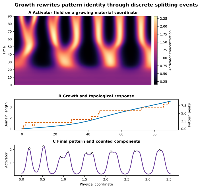
The representative calculation starts from small seeded perturbations around the homogeneous state and grows the domain with rate $0.01$ until $t=90$ . The physical length reaches approximately $3.562$ times its initial value.

The final profile contains nine detected peaks. Across the saved history the tracker records eleven birth or death events, while the final dominant cosine mode is 13. The final spectral entropy is approximately $0.323$ , showing that the state is structured but not a pure single harmonic. The smallest state value remains positive at about $0.153$ .

These numbers should be read as a sequence, not as a contradiction with the fixed-domain mode-5 baseline. Mode 5 describes the initial linear preference on the original length. By the end, the physical domain is much longer, nonlinear saturation has occurred, and the observed profile has travelled through several event-generating regimes.

Figure 1 makes the timing visible. Long stretches can preserve the same peak count even while length changes. A later split can occur over a relatively short interval. This is why comparing only the first and last image loses the mechanism: two simulations with the same final count may have very different histories and sensitivities.

A phase atlas rather than one attractive trajectory

A single run is useful for explanation but weak evidence for a two-parameter claim. The study therefore varies growth rate together with a kinetic-margin parameter that moves the reaction system relative to the instability boundary.

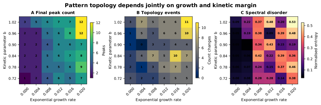
Phase atlas showing final peak count and topology-event behaviour across growth rate and kinetic margin. — **Figure 2.** Growth-rate × kinetic-margin atlas. Numeric labels and boundary annotations supplement colour, so the regimes remain interpretable without relying on hue alone.

The atlas shows why “faster growth gives more peaks” is too simple. Increasing growth creates more physical room, but it also increases dilution and changes the time available for an unstable mode to amplify. Near the kinetic boundary, a disturbance may never become prominent enough to count. Deeper inside the unstable region, growth can create repeated splitting. In another part of the grid, a transient feature forms and is later lost.

The meaningful object is consequently a regime map:

persistence: pattern features remain identifiable while stretching;
insertion or splitting: new peaks appear between existing ones;
loss or merging: peaks fall below prominence or combine;
suppression: perturbations do not form a robust pattern during the simulated window.

These labels are descriptions of the declared simulator and detection rule. They are not developmental-biological phenotypes.

Verification before interpretation

Pattern-forming PDEs are particularly good at producing persuasive numerical artefacts. A coarse grid can change which modes are resolved; a large time step can damp or amplify structure; a peak threshold can manufacture events. The verification panel therefore belongs in the main evidence, not in an invisible appendix.

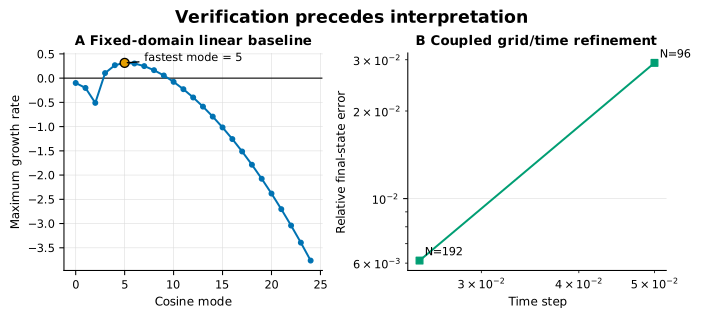
Verification figure comparing fixed-domain dispersion, grid and time-step refinement, mass residual, and minimum state. — **Figure 3.** Independent checks: analytical linear baseline, refinement trend, balance residual, and positivity. Verification narrows numerical doubt but does not validate a biological mechanism.

Three coupled checks are reported.

A common comparison configuration is rerun at coarse, reference, and fine resolution. Relative $L^2$ error against the fine solution falls from approximately $2.93\times10^{-2}$ to $6.12\times10^{-3}$ before reaching the reference zero by definition. The compared configurations retain the same final peak count of three.

The representative story has nine final peaks because it is a different declared story configuration from the dedicated refinement case. Keeping these roles separate matters: refinement should compare like with like, while the story should illustrate the phenomenon selected for explanation.

Balance residual

On a growing domain, a naive “mass must stay constant” check is wrong because reaction, dilution, and physical volume all contribute. The implementation instead evaluates the residual of the model-implied balance. Its maximum absolute value is about $1.3\times10^{-3}$ across refinement levels. That is not mathematical proof, but it supplies an order-of-magnitude diagnostic that would expose a missing growth or diffusion term.

Positivity

The minimum activator or inhibitor concentration remains above zero in the reported runs. Positivity is both a physical sanity condition for this interpretation and a numerical diagnostic. It cannot establish accuracy by itself: a smooth positive wrong solution is still wrong. That is why it is reported beside convergence and the analytical dispersion relation.

What changes if the peak detector changes?

Peak prominence is part of the measurement model. Tightening it can reclassify small shoulders as “no event”; relaxing it can split noisy ripples into false peaks. A responsible reading therefore treats exact event count as conditional on the declared detection rule.

The more stable claims are qualitative and multi-view:

domain growth moves the admissible spatial scale;
dilution competes with amplification;
the nonlinear history contains distinct intervals of persistence and event formation;
a fixed-domain linear mode does not determine final peak count;
within the tested range, the reported regimes survive the numerical checks used here.

A stronger future analysis would report persistence diagrams of extrema across prominence thresholds, or use continuation of nonlinear patterned branches on growing domains. That would reduce dependence on one detector without pretending that “pattern identity” is observer-free.

What the experiment does not establish

This calculation does not show that a particular tissue uses Schnakenberg kinetics. It does not estimate a biological growth rate, diffusion coefficient, or molecular concentration. It assumes one-dimensional uniform growth, no-flux endpoints, two reacting fields, and synthetic initial perturbations. Cell rearrangement, anisotropic growth, mechanical feedback, receptor binding, gene regulation, and measurement noise are absent.

The result is therefore a verified mechanism study:

In the declared growing-domain reaction–diffusion model, geometric growth changes pattern topology through the combined effects of evolving wavelength, dilution, and nonlinear history.

Moving from that statement to an organism-specific claim would require independently measured geometry, kinetics, transport scales, molecular readouts, and competing-mechanism tests.

Why this is a useful modeling example

The example joins material that is usually taught in separate chapters.

Linear algebra and stability analysis produce the dispersion baseline. A coordinate transformation exposes how geometry enters the PDE. Spectral numerical methods implement the no-flux diffusion operator. Signal processing turns a field into measurable events. Refinement and balance checks constrain numerical interpretation. Finally, scientific writing keeps the mechanism claim inside the synthetic model.

That chain is more valuable than an attractive stripe plot because every step can be challenged. Change the growth law, repeat the atlas. Change the prominence rule, examine event persistence. Change the solver, compare fields. Add data only when its provenance and role are explicit.

References

A. M. Turing, “The chemical basis of morphogenesis,” Philosophical Transactions of the Royal Society B, 1952. doi:10.1098/rstb.1952.0012.
S. Paul, J. Adetunji, and T. Hong, “Widespread biochemical reaction networks enable Turing patterns without imposed feedback,” Nature Communications, 2024. doi:10.1038/s41467-024-52591-0.
C. Husbands et al., “A diffusible small-RNA-based Turing system dynamically coordinates organ polarity,” Nature Plants, 2024. doi:10.1038/s41477-024-01634-x.
J. D. Murray, Mathematical Biology II: Spatial Models and Biomedical Applications, 3rd ed., Springer, 2003. doi:10.1007/b98869.