
A genetic switch can spend a long time looking stable and then change state in a short, noisy burst. That contrast makes the phrase “How often does it flip?” sound simpler than it is. The probability depends on what counts as a flip, when observation stops, which stochastic model is being simulated, and whether the numerical method can resolve an event that may occur only rarely.
This project began with an ambitious comparison: test adaptive multilevel splitting against direct Gillespie simulation and an error-controlled forward-flux baseline. The literature review changed that plan before the comparison was run. Rare-event sampling on genetic and biochemical switches is not an empty field, and a generic demonstration that enhanced sampling can outperform brute force would repeat established work. The review therefore led to REFRAME: narrow the question before computing.
The defensible question is narrower: on one fixed exclusive-toggle continuous-time Markov chain, can a future benchmark expose where an estimator loses calibration as its progress coordinate is deliberately degraded, while charging every method for setup and sampling? That future question requires a trustworthy reference and a verified direct-simulation baseline first.
This article reports only that foundation. It is a synthetic, low-copy Phase-1 smoke study. A finite-state projection (FSP) at molecule cap 20 brackets the declared fixed-horizon hit probability between and , with overflow probability . A seeded direct SSA run records hits among trajectories, an estimate of , with a 95% Wilson interval from to . In 32 smaller independently seeded batches, 30 Wilson intervals intersect the FSP bracket. Structural invariants and a hand-calculable special case provide separate numerical checks.
Those are the complete positive claims. No adaptive multilevel splitting or FFPilot result appears here. There is no rare-event speedup, no biological validation, and no final rarity ladder. The event probability is roughly one quarter in this smoke configuration, so it would be especially misleading to present the calculation as evidence that a difficult rare-event regime has already been solved.
What Phase 1 established
| Question | Finding | Why it matters |
|---|---|---|
| What system was used? | A synthetic low-copy exclusive-toggle CTMC | It is a controlled numerical case, not a named biological circuit. |
| What counts as the event? | First entry into a declared -dominant set by | The result is a fixed-horizon hit probability, not a stationary rate or MFPT. |
| Was cap 18 sufficient? | No; it exceeded the fixed overflow and bracket tolerance | The failed truncation shows why the state space had to be enlarged. |
| What did cap 20 provide? | , overflow | It gives a tight reference bracket for this smoke event. |
| What did direct simulation give? | Its Wilson interval intersects the FSP bracket. | |
| Did the smaller batches agree perfectly? | No; 30 of 32 intervals intersected the bracket | The two misses expose ordinary finite-sample variation. |
The wording in the last column is deliberate. An interval intersecting a reference does not prove that every numerical detail is correct. Agreement with structural and analytic checks does not validate a biochemical mechanism. A very narrow truncation bracket does not turn a moderately probable event into a rare one. Each piece of evidence answers one question and leaves several others open.
Why the literature changed the question
The original attraction of the project was computational. If direct simulation waits through many ordinary reaction events before observing a transition, a splitting or importance-sampling method may concentrate effort near transition pathways. That idea is important, but it is not new.
Allen, Warren, and ten Wolde introduced forward-flux sampling for rare switching in biochemical networks and applied it to mutually repressing genetic switches in 2005. Allen, Frenkel, and ten Wolde then compared several interface and path-sampling schemes on a genetic switch in 2006. Morelli and colleagues studied reaction-coordinate quality and committor structure for flips in general and exclusive genetic switches in 2008. These papers already occupy the most obvious territory: access to rare flips, method comparison, and the role of a progress coordinate.
The overlap extends beyond forward-flux sampling. Roh and colleagues developed a state-dependent doubly weighted stochastic simulation algorithm for biochemical rare events, including a bistable lac-operon switch in 2011. Cao and Liang compared adaptively biased sequential importance sampling with finite-buffer chemical-master-equation calculations in 2013. Tse and colleagues used weighted-ensemble string sampling to study how DNA-binding kinetics changes noise-induced switching paths in 2015, and later combined rare-event sampling with coarse-grained landscape and phenotype-transition analysis in 2018.
Two other strands matter directly to experimental design. Rolland and Simonnet showed in simple models that adaptive multilevel splitting can behave poorly when the reaction coordinate is inadequate in 2015. Cao, Terebus, and Liang developed multi-finite-buffer chemical-master-equation calculations with controlled truncation for systems that include genetic toggles in 2016. Klein and Roberts added automatic full-phase error control to forward-flux sampling and tested it on master-equation models including a genetic toggle in 2020.
Together, these ten primary works make three broad points established literature rather than local discoveries. First, rare switch events in biochemical and genetic networks can be sampled with interface, weighted-ensemble, or importance-sampling approaches. Second, error control, reaction-coordinate quality, and setup cost are central to a fair comparison. Third, a tractable low-copy toggle may admit a finite-state master-equation reference that is stronger than simply declaring a very large Monte Carlo run to be truth.
The remaining opening is therefore diagnostic, not triumphant. A useful benchmark could freeze several progress coordinates in advance, degrade them in a controlled way, compare empirical interval coverage and error at matched total compute, and record the boundary where the method becomes unreliable. Phase 1 does not execute that benchmark. It only asks whether the model, event, direct simulator, uncertainty calculation, and finite-state reference can agree in a tractable regime.
The synthetic exclusive toggle
The state is
where and are total low-copy protein counts and the shared operator state is
means the operator is unbound, means one protein is bound, and means one protein is bound. Because there is one shared operator, simultaneous - and -binding is excluded. A bound protein remains included in its species total. That accounting choice matters when degradation is defined: only free proteins degrade in this smoke model.
The reaction channels are production, free-protein degradation, monomer binding, and unbinding. In schematic form,
plus transitions among , -bound, and -bound operator states. When is bound, production is multiplied by a leak fraction; when is bound, the same rule represses production. Binding to the shared operator therefore creates the mutually repressing architecture.
The fixed synthetic parameters are symmetric. Both unrepressed production rates are ; the leak fraction is ; both degradation rates are ; both binding coefficients are ; and both unbinding rates are . The initial state is
so the system begins -dominant with bound to the operator.
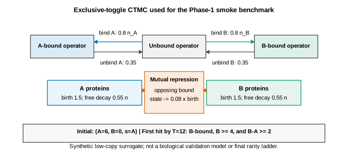
This model is intentionally small. It does not name an organism, promoter, plasmid, copy-number calibration, or experimentally measured rate. It omits mRNA, transcriptional bursts, translation delay, cell growth and division, extrinsic noise, resource competition, and evolutionary stability. Its purpose is numerical traceability: every legal state is discrete, every transition has a declared propensity, and the low copy numbers make an independently bounded finite-state calculation feasible.
That purpose is different from the earlier site study on qualitative noise-induced switching. Here the primary observable is not a stationary landscape or an unconstrained mean first-passage time. It is one sharply defined fixed-horizon event.
What exactly counts as a flip?
Let the observation horizon be . The target set is
The event is the first visit to on or before :
All three clauses matter. Requiring prevents one or two molecules from being called a switched state. Requiring imposes an abundance margin rather than accepting a tie. Requiring to occupy the operator incorporates the regulatory state rather than classifying by protein counts alone.
Once a trajectory first enters , it is counted as a hit even if it would later leave. The quantity under study is therefore
It is not the same object as a stationary transition rate. It is not automatically the reciprocal of a mean first-passage time. It is also not a probability per unit time. Those quantities may be related under additional assumptions or limiting regimes, but mixing them would make the numerical comparison ill posed.
Fixing the event before simulation is especially important in rare-event work. If a target threshold, time horizon, or basin definition is adjusted after seeing which trajectories succeed, the estimator is no longer answering the preregistered question. In this Phase-1 run, model parameters, initial state, event definition, truncation tolerance, seeds, and budgets were fixed in the smoke configuration.
Direct Gillespie simulation as a baseline
For a continuous-time Markov chain with state-dependent reaction propensities , the direct stochastic simulation algorithm draws an exponential waiting time with total rate
and chooses reaction with probability . The state is updated and the process repeats until the trajectory hits or reaches .
For trajectory , define the Bernoulli indicator
The naive Monte Carlo estimator is
It is transparent and, for the declared CTMC, directly simulates the target event. Its sampling variance is
The relative standard error behaves approximately like
This formula explains why direct Monte Carlo becomes unattractive when is extremely small: obtaining a useful number of hits requires to grow roughly like . But Phase 1 does not demonstrate that difficulty. With , the event is common enough for an ordinary baseline check.
The seeded aggregate run used trajectories and obtained
A binomial interval is more informative than reporting only five decimal places. The study uses the Wilson interval. For confidence level , with normal quantile , the Wilson centre and half-width are
At 95% confidence, the recorded interval is
This is sampling uncertainty for the direct estimator. It does not include model-form error, biological parameter uncertainty, or an unknown mismatch between the synthetic CTMC and a real genetic circuit.
Building a reference without declaring Monte Carlo to be truth
To check the direct simulation, Phase 1 uses an independently assembled finite-state projection. Choose a cap and enumerate legal non-target states satisfying
along with valid , -bound, and -bound occupancy states. Add two absorbing sinks. The first collects probability when a transition enters . The second collects probability when a path exits the rectangular molecule-count truncation.
If is the resulting finite generator and places all mass at , then the transient distribution at time is obtained from the matrix exponential,
Let be mass in the target sink and be mass in the overflow sink. Every path counted in the target sink is a genuine hit of the untruncated CTMC, so it supplies a lower bound. In the most conservative case, every overflowed path could later hit the target before . Therefore
The width of this bracket is exactly the overflow probability, apart from numerical rounding. This construction does not guess the unobserved tail. It records the maximum amount by which omitted states could change the hit probability.
That distinction is why the overflow tolerance was not relaxed after a failed attempt. A finite-state calculation is only useful as a reference if its declared error control survives contact with the chosen state space.
Why cap 18 was rejected
With , the calculation produced the bracket
with overflow probability about . The preregistered maximum bracket width was , so cap 18 failed. The calculation was not relabelled as “close enough,” and the tolerance was not enlarged after the result was seen.
The next attempt increased the count cap to 20. It produced
and hence
Rounded to ten decimal places, the Phase-1 reference bracket is
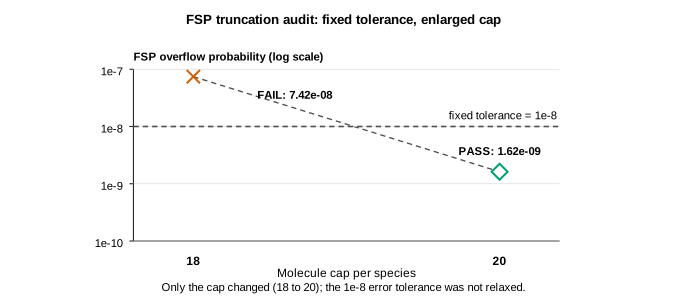
Keeping the failure is more than housekeeping. If only the successful cap were shown, a reader could not tell whether the state space was enlarged according to a fixed rule or whether a tolerance was adjusted until the desired label appeared. The retained attempt documents which control failed and what changed: the cap increased; the criterion did not.
Cap 20 is not being treated as the unbounded state space. Its value comes from the probability bracket, not from the label on the cap. The retained-state calculation gives the lower bound, and adding the unresolved overflow mass gives the upper bound. Once that gap is , the omitted states can change the declared hit probability by no more than that amount under this construction. A larger cap might narrow the bracket further, but it would not alter the scale of the comparison with the much wider SSA interval.
Comparing the bounded reference with seeded SSA
The FSP midpoint is approximately . The seeded direct estimate is , about above that midpoint. Reporting that absolute difference without sampling uncertainty would exaggerate its meaning. With only 6000 Bernoulli trials, an estimate need not land inside a reference bracket whose width is on the order of .
The appropriate smoke question is whether the direct interval is compatible with the reference. It is:
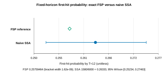
The two calculations fail differently. Direct SSA has Monte Carlo sampling error but does not truncate molecule counts. The FSP has a controlled state-space truncation whose omitted mass is made explicit, while the matrix-exponential calculation is deterministic for the declared finite generator. Agreement therefore checks more than running the same code twice. It compares independently structured routes to the same fixed-horizon probability.
Still, one agreement is not enough to calibrate an interval procedure. The aggregate interval could intersect the reference by chance, and a single seed hides run-to-run variation. Phase 1 therefore included a small batch diagnostic.
Thirty intersections out of thirty-two
The diagnostic used 32 independent seeded batches, each containing 300 direct SSA trajectories. Every batch produced its own hit fraction and 95% Wilson interval. The predefined diagnostic called a batch an intersection when its interval overlapped the rigorous FSP bracket.
Thirty of the 32 intervals intersected. Two did not. In the figure, open circles distinguish intersections and cross markers retain the misses.
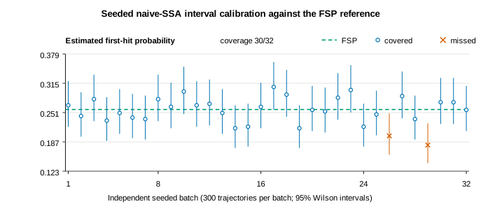
Why not announce 93.75% empirical coverage? The arithmetic is correct,
but the word “coverage” carries a repeated-sampling meaning. Thirty-two batches are too few to estimate a nominal 95% coverage probability tightly. Moreover, the diagnostic is based on interval intersection with a narrow probability bracket, rather than an exactly represented scalar truth. Here the bracket is so tight that the difference is negligible for visual interpretation, yet the distinction should remain explicit.
The two misses are informative rather than embarrassing. At 300 trajectories per batch, binomial variation is large enough that some intervals need not include a fixed probability. Removing those seeds would convert a calibration check into selection on the outcome. Preserving them makes the diagnostic fully visible and keeps the article from implying perfect behavior.
Why the numerical verification is credible
The emitted reaction channels have positive rates and preserve valid nonnegative states, including occupancy-dependent repression and free-protein degradation. The finite generator is conservative, with nonnegative off-diagonal rates and nonpositive diagonal entries. A separate calculation compares the FSP result with the analytic single-birth first-hit probability
in a special case where that answer is known. In the same special case, seeded SSA gives a Wilson interval containing the analytic probability, while repeating the calculation with the same fixed seed reproduces its result.
Together, these comparisons connect general invariants to a known special case and then to the reported smoke calculation. They do not establish that the synthetic rates describe a real cell, exclude every possible numerical error, or validate AMS or FFPilot, because those methods are not part of the Phase-1 result. They also establish no result on the final rarity ladder. Numerical agreement strengthens this baseline without widening the scientific claim.
Established knowledge versus the local smoke result
This separation is the central scientific distinction for the project.
Established in the cited primary literature: rare-event methods have been applied to biochemical and genetic switching; interface placement and reaction-coordinate quality matter; weighted and biased sampling can access transition probabilities and pathways; setup and sampling uncertainty require error control; and finite-state master-equation calculations can provide controlled references in tractable regimes.
Observed locally in Phase 1: for one synthetic low-copy exclusive toggle and one fixed-horizon -dominant first-hit event, the cap-20 FSP bracket is –, seeded direct SSA gives with Wilson interval –, 30 of 32 smaller batch intervals intersect the reference, and the stated verification checks pass.
Not observed locally: any result for adaptive multilevel splitting, FFPilot, importance sampling, progress-coordinate degradation, matched-compute efficiency, rare-event speedup, a preregistered rarity ladder, stationary switching rates, mean first-passage-time accuracy, or biological data.
The distinction prevents a subtle but common reasoning error. A method can be well established in literature without having been tested in this Phase-1 study. Conversely, a local baseline can be internally consistent without being novel or biologically realistic. Combining the two into “we proved rare-event sampling works for genetic switches” would attribute other researchers’ results to a small smoke calculation.
Why this event is not yet the promised rare event
The title asks how rare a flip is, but the Phase-1 answer is intentionally mundane: under this configuration and horizon, the declared target is reached with probability about . That is roughly one hit in four trajectories, not one in a million.
This moderate probability is useful for software validation. Direct simulation produces many hits, so implementation mistakes can be detected without an enormous compute budget. The finite-state truncation is also tractable, so its overflow mass can be driven below a tight fixed tolerance. These properties make the regime a good smoke test.
They make it a poor basis for a speedup claim. When events are common, a rare-event method can spend more on pilot runs, interfaces, replicas, or coordinate design than direct SSA spends collecting hits. The literature review turned the study toward total-cost accounting, but Phase 1 does not measure that accounting. It would be invalid to take the passing reference comparison and infer that an enhanced sampler will later be faster.
Nor does the current probability define a “flip rate.” Shortening or lengthening , changing the target margin, changing the required operator occupancy, or changing the starting state would produce a different probability. The future rarity ladder must freeze those design choices and alter only preregistered regime controls. Until that ladder is run, the project has no empirical statement about how estimator reliability changes with rarity.
What the next benchmark must test
The reframed research design calls for several ingredients that are future work, not implied results:
- one fully specified exclusive-toggle CTMC and fixed event definition across a preregistered rarity ladder;
- naive SSA, adaptive multilevel splitting, and an error-controlled forward-flux baseline evaluated at matched total compute;
- a small fixed family of progress coordinates, ranging from mechanistically informed to deliberately misspecified;
- reference probabilities from error-controlled finite-state calculations wherever tractable, with separately seeded direct simulation only where that reference is infeasible;
- empirical interval coverage, relative bias or RMSE, variance per total compute, and failed-run rate as primary diagnostics;
- all pilot, interface-selection, training, and tuning cost charged to the method that incurs it; and
- a non-rare regime in which enhanced sampling is not assumed to help.
This is a plan, not an achievement list. No item involving AMS, FFPilot, coordinate stress testing, matched-compute comparison, or the final ladder has been executed in the evidence reported here. The literature review supplies the reason to run such a benchmark; it does not supply its outcome.
The future benchmark could also fail to produce a useful boundary. If preregistered coordinate degradation does not lead to a reproducible change in calibration, or if total-cost accounting leaves no practically meaningful result beyond the established literature, the honest conclusion would be a null or stopped project. Reframing protects against manufacturing novelty from a generic speedup demonstration.
What Phase 1 contributes
The contribution is procedural and bounded. The event is written as a first-hit set rather than an informal visual flip. The direct estimator has a named uncertainty interval rather than an unqualified decimal. The finite-state reference exposes overflow mass rather than hiding truncation. The failed cap-18 calculation remains visible. Independent seeds expose two missed batch intervals, while structural invariants and an analytic special case support the baseline. The article states what was not run alongside what passed.
These choices do not make the underlying methods new. They make the next result easier to interpret. If a later estimator disagrees with the cap-20 reference in a tractable regime, investigators can ask whether the problem lies in coordinate choice, sampling variance, interval construction, or implementation. If direct SSA and the reference had failed to agree here, building an elaborate rare-event comparison on top would have been premature.
The most important number may therefore be neither nor . It may be 18: the cap that failed and was preserved. A reliability study earns credibility by retaining the point where a control did not pass, then changing one justified input—the state-space cap—without moving the threshold.
How to read the figures
The four figures form a logical sequence rather than decoration. Figure 1 declares the synthetic state model and target event. Figure 2 records the truncation failure and the controlled correction. Figure 3 compares two independently structured probability calculations. Figure 4 exposes run-to-run interval variation and retains the misses. Read in that order, they move from question to reference, baseline comparison, and uncertainty diagnostic.
None is a biological diagram in the experimental sense. The network schematic represents the mathematical CTMC. None shows AMS particles, forward-flux interfaces, a rarity ladder, or a speedup curve because those experiments were not run in Phase 1. The captions say this directly so that an isolated image does not inherit a stronger claim than the article.
A compact answer to the title
For the declared synthetic low-copy model, start, target, and horizon, the best Phase-1 answer is the FSP bracket
Seeded direct simulation is compatible with that reference at its stated uncertainty: hits in trajectories give , with a 95% Wilson interval of . Thirty of 32 smaller batch intervals intersect the bracket.
That answer is about one smoke event. It does not say how often a real genetic switch flips, how fast an enhanced sampler would be, whether a progress coordinate is reliable, or what happens along the final rarity ladder. The literature review shows that those broader computational questions have substantial precedent and require a narrower reliability test.
So the project ends Phase 1 with a useful asymmetry: the numerical reference is tight, while the scientific claim is intentionally small. That is the right direction. Precision in a calculation should narrow uncertainty about the declared model; it should not widen the scope of what the model is allowed to represent.
References
- Allen, R. J., Warren, P. B., & ten Wolde, P. R. (2005). Sampling Rare Switching Events in Biochemical Networks. Physical Review Letters, 94, 018104. https://doi.org/10.1103/PhysRevLett.94.018104
- Allen, R. J., Frenkel, D., & ten Wolde, P. R. (2006). Simulating Rare Events in Equilibrium or Nonequilibrium Stochastic Systems. The Journal of Chemical Physics, 124, 024102. https://doi.org/10.1063/1.2140273
- Morelli, M. J., Tanase-Nicola, S., Allen, R. J., & ten Wolde, P. R. (2008). Reaction Coordinates for the Flipping of Genetic Switches. Biophysical Journal, 94, 3413–3423. https://doi.org/10.1529/biophysj.107.116699
- Roh, M. K., Daigle, B. J., Jr., Gillespie, D. T., & Petzold, L. R. (2011). State-Dependent Doubly Weighted Stochastic Simulation Algorithm for Automatic Characterization of Stochastic Biochemical Rare Events. The Journal of Chemical Physics, 135, 234108. https://doi.org/10.1063/1.3668100
- Cao, Y., & Liang, J. (2013). Adaptively Biased Sequential Importance Sampling for Rare Events in Reaction Networks with Comparison to Exact Solutions from Finite Buffer dCME Method. The Journal of Chemical Physics, 139, 025101. https://doi.org/10.1063/1.4811286
- Rolland, J., & Simonnet, E. (2015). Statistical Behaviour of Adaptive Multilevel Splitting Algorithms in Simple Models. Journal of Computational Physics, 283, 541–558. https://doi.org/10.1016/j.jcp.2014.12.009
- Tse, M. J., Chu, B. K., Roy, M., & Read, E. L. (2015). DNA-Binding Kinetics Determines the Mechanism of Noise-Induced Switching in Gene Networks. Biophysical Journal, 109, 1746–1757. https://doi.org/10.1016/j.bpj.2015.08.035
- Cao, Y., Terebus, A., & Liang, J. (2016). Accurate Chemical Master Equation Solution Using Multi-Finite Buffers. Multiscale Modeling & Simulation, 14, 923–963. https://doi.org/10.1137/15M1034180
- Tse, M. J., Chu, B. K., Gallivan, C. P., & Read, E. L. (2018). Rare-Event Sampling of Epigenetic Landscapes and Phenotype Transitions. PLOS Computational Biology, 14, e1006336. https://doi.org/10.1371/journal.pcbi.1006336
- Klein, M. C., & Roberts, E. (2020). Automatic Error Control during Forward Flux Sampling of Rare Events in Master Equation Models. The Journal of Chemical Physics, 152, 035102. https://doi.org/10.1063/1.5129461