From Pixels to Patrols: Why Calibration Changes a Synthetic Patrol Plan

Programme status — 30 August 2026. The official AI4Nature@AVSS 2026 programme lists From Pixels to Patrols: A Calibration-Aware Sensor Fusion Pipeline for Camera-Trap-Driven Anti-Poaching Resource Allocation as Paper ID 7 in Oral Session 1A on 31 August 2026. The presentation is scheduled for tomorrow; it has not yet occurred. Proceedings publication, an IEEE Xplore record, and a DOI are pending.

Evidence boundary. Every numerical value below is manuscript-reported from controlled synthetic experiments over twenty separately seeded networks with 400 cells each. I did not independently rerun the code or reproduce those values for this Blog note. The study contains no real camera-trap images, patrol logs, protected-area deployment, or field-effectiveness validation.

The official programme lists Ka Hin Chan, Long Nam Ao, Weng Kin Loi, Long Tin Tse, and Sok Kin Cheng as the authors. Their study begins with a deceptively simple observation: a classifier score can become an operational quantity even when nobody explicitly calls it one.

Suppose a camera-trap model assigns a probability to a human-presence class. A downstream system may sum those probabilities within spatial cells, rank the cells, and allocate a fixed number of patrol hours. If a score of $0.8$ behaves empirically like an event rate of $0.5$ , the error does not stop at the classifier. It changes the estimated spatial risk field and can move scarce resources to different cells.

The manuscript asks how that probability-to-decision chain behaves in a controlled setting. It does not ask whether an operational anti-poaching programme is effective. The human-presence class is a risk proxy, not a direct poacher label; authorised staff, tourists, researchers, vehicles, routes, seasonality, travel time, safety, and local conservation knowledge are outside the synthetic experiment.

One chain, several separate questions

The pipeline has five conceptual stages:

a four-class synthetic classifier emits a probability vector for each image;
four disjoint labelled batches serve calibrator fitting, metric evaluation, interval calibration, and deployment checking;
temperature scaling adjusts the full multiclass distribution, while a second monotone map targets the named risk-proxy class;
image probabilities become per-cell expected counts and realised-count intervals;
a constrained allocator maps those cell summaries to patrol time.

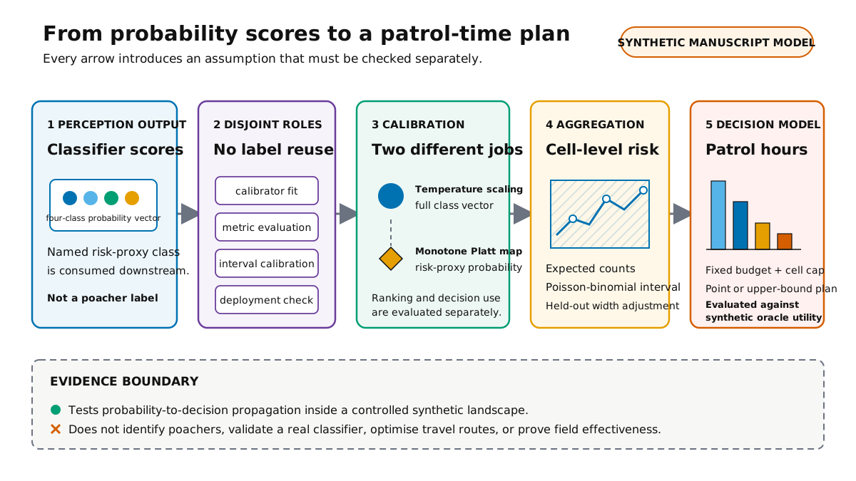
Five-stage diagram connecting synthetic classifier probabilities, disjoint data roles, calibration, cell-level aggregation, and constrained patrol allocation, with a field-validation boundary. — **Figure 1.** A newly drawn editorial explanation of the manuscript pipeline, not a figure extracted from the supplied paper. The dashed boundary matters: the chain is tested inside a synthetic landscape and does not establish real patrol effectiveness.

Each stage answers a different question. Multiclass calibration asks whether confidence values across predicted labels correspond to empirical frequencies. Task calibration asks whether the particular class probability consumed by the allocator is reliable. Count aggregation asks how image-level uncertainty accumulates within a cell. Allocation asks how errors in those counts change a decision under a declared utility function.

Combining all four into one headline such as “better calibration improves conservation” would skip most of the causal chain. The paper instead evaluates intermediate quantities and an explicitly synthetic decision objective.

Why the data roles are separated

Calibration can look successful when the same labels influence both the fitted transformation and its evaluation. The manuscript avoids this direct leakage by generating four conditionally independent batches from one latent synthetic landscape:

the fit batch estimates calibration parameters;
the evaluation batch reports ECE, Brier score, and negative log likelihood;
the interval-calibration batch chooses a predictive-width adjustment;
the deployment batch checks realised counts and decision performance.

This separation is a methodological strength. It prevents the deployment check from doubling as a tuning set. It does not make the synthetic cells independent in every scientific sense: they still share the same landscape-generating assumptions, spatial correlation model, class biases, and observation model. The result is a clean test of internal behaviour, not evidence that the same transformations will survive a new reserve, season, camera, or classifier.

Two calibration jobs

Let $\boldsymbol{\pi}_j$ be the four-class probability vector for image $j$ , and let $\ell_j=\log \boldsymbol{\pi}_j$ . Temperature scaling fits one positive scalar $T$ :

\widehat{T} =\arg\min_{T>0} -\sum_{j\in C_{\mathrm{fit}}} \log\left[\operatorname{softmax}(\ell_j/T)\right]_{y_j}.

Because division by one scalar preserves the ordering of class logits, temperature scaling can soften or sharpen confidence without changing the predicted class. It is a compact correction for global overconfidence, but the patrol allocator does not consume only the top-label confidence. It consumes the probability of one named risk-proxy class $K$ .

The manuscript therefore fits a second monotone transformation,

q_j =\sigma\!\left(a\,\operatorname{logit}(\pi_{jK})+b\right), \qquad a>0,

where $q_j$ is the task-calibrated risk-proxy probability. The positive-slope constraint preserves the class score ordering while allowing the probability scale to change.

This distinction is easy to miss. A classifier may have acceptable top-label calibration yet still overstate or understate the probability of the one class that drives a downstream count. Conversely, better calibration of that one class does not prove that every class or every use of the model is calibrated.

The paper reports expected calibration error, but ECE depends on binning and implementation details. Until the implementation and a stable revision are available for inspection, this Blog treats the reported ECE values as manuscript evidence rather than an independently audited statistic.

From image probabilities to uncertain cell counts

For cell $i$ , the task-calibrated point estimate is the sum

\widehat z_i=\sum_{j\in D_i}q_{ij}.

That number is an expected count, not a realised count and not a probability that the cell contains a poacher. The manuscript models a realised synthetic count as a sum of Bernoulli variables,

Z_i=\sum_{j\in D_i}B_{ij}, \qquad B_{ij}\sim\operatorname{Bernoulli}(q_{ij}),

which produces a Poisson-binomial distribution when the probabilities differ. Dynamic programming gives a base interval. A held-out calibration batch then selects a non-negative integer margin to widen the interval before deployment evaluation.

The manuscript explicitly declines a distribution-free conformal guarantee. Coverage remains conditional on the probability model and on how well the interval-calibration batch represents deployment. That is the correct boundary: an empirical coverage result in a simulator is not a universal theorem about future camera networks.

The allocation model

The fixed-budget experiment uses a diminishing-return utility

u_i(\tau_i,z_i) =z_i\left(1-e^{-\lambda\tau_i}\right),

subject to a total patrol-time budget and a per-cell cap. More estimated risk initially attracts more time, but the marginal gain within one cell decreases. The optimiser therefore distributes time across cells rather than placing the entire budget at the largest point estimate.

Policies based on raw, temperature-scaled, task-calibrated, and predictive-upper counts are compared with a synthetic oracle. Regret is the oracle utility minus the utility obtained by the tested policy, evaluated on the simulator’s expected field.

This construction makes the decision consequence measurable. It is also highly stylised. It does not include travel routes, ranger starting locations, terrain, access restrictions, uncertain detection after patrol, adversarial adaptation, staff safety, or the harm of treating ordinary human presence as suspicious. Those omissions prevent the utility score from being read as an operational recommendation.

What the manuscript reports

The following values come from the author-provided camera-ready manuscript and have not been independently reproduced here.

Across twenty synthetic 400-cell networks, the manuscript reports:

top-label ECE changing from $0.341\pm0.010$ for raw scores to $0.048\pm0.010$ after temperature scaling;
risk-proxy ECE changing from $0.111\pm0.013$ raw, to $0.057\pm0.005$ after temperature scaling, and $0.017\pm0.005$ after task calibration;
oracle-relative patrol regret changing from $2.64\pm0.51\%$ for the raw plan to $0.54\pm0.21\%$ after temperature scaling and $0.33\pm0.08\%$ after task calibration;
base interval coverage of $0.877\pm0.028$ and held-out calibrated coverage of $0.932\pm0.020$ for a nominal $0.90$ interval;
an $87.46\pm2.20\%$ closure of the raw-policy regret gap after task calibration.

The manuscript uses $\pm$ notation for across-seed summaries; this Blog calls those quantities reported dispersion and does not relabel them as confidence intervals. The precise aggregation should be checked against the released implementation or an accompanying result table.

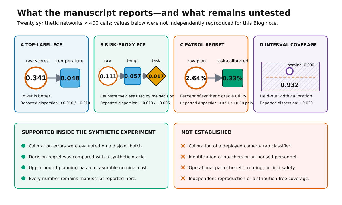
Four-card summary of manuscript-reported top-label calibration error, risk-proxy calibration error, patrol regret, and interval coverage, followed by supported and unsupported claim boundaries. — **Figure 2.** A new editorial summary drawn from numerical values reported in the manuscript. Lower ECE and regret are favourable inside the simulator; the coverage point is compared with a nominal 0.90 level. No value in this figure was independently reproduced for this Blog note.

The result pattern is coherent with the paper’s question. Correcting the full class vector helps, and calibrating the exact probability used by the decision rule helps further. The study therefore demonstrates a decision-stage consequence of probability scale inside its declared synthetic protocol.

It does not demonstrate that a real camera-trap classifier will exhibit the same amount of miscalibration or the same improvement. The simulator deliberately creates an overconfident regime using class bias and noisy logits. A deployed model may fail differently through domain shift, unseen species, poor illumination, camera hardware, habitat, human activity, or changes in class prevalence.

Why an upper bound is not automatically safer

The manuscript also compares a task-calibrated point plan with a plan based on predictive upper endpoints. Under the selected upper-risk stress field, the upper-bound plan is protective by construction. Under the nominal field, it can over-concentrate resources and incur additional cost.

This is a useful negative result. “Use the upper confidence bound” is not a free robustness principle. Its value depends on the loss assigned to missed events, patrol hours, and false concentration of effort. A real decision would need stakeholder-defined costs and operational constraints rather than a generic preference for conservative numbers.

What this study does not establish

The manuscript itself identifies synthetic evaluation as the main limitation. The following statements would go beyond the available evidence:

that the pipeline detects poachers;
that a human-presence class separates authorised from unauthorised people;
that a deployed classifier is calibrated at a named protected area;
that the synthetic utility represents animals saved, incidents prevented, or ranger safety;
that the interval has distribution-free coverage;
that upper-bound planning is universally robust;
that the reported values have been independently reproduced;
that the paper has already been presented, published in proceedings, indexed by IEEE Xplore, or assigned a DOI.

Real deployment would require lawful and ethical governance of imagery involving people, records of authorised presence, local review, secure handling of sensitive conservation locations, route-aware planning, monitoring for seasonal and hardware shift, and repeated calibration checks. Public communication should never expose patrol routes or vulnerable-species coordinates.

Reproducibility and publication status

The supplied six-page PDF says that the implementation is available in a project repository, but it contains no repository URL. I did not verify a public code revision, dependency environment, complete seed list, machine-readable result table, or output manifest. The numerical claims therefore remain manuscript-reported.

The PDF metadata states that it was certified by IEEE PDF eXpress. IEEE’s conference guidance explains that PDF eXpress checks or converts files for IEEE Xplore compatibility; that metadata is not an IEEE Xplore publication record.

The publication pathway is nevertheless stronger than a vague possibility. The AI4Nature call for papers says accepted papers will be included in the AVSS 2026 proceedings and published in IEEE Xplore, with at least one full registration covering each accepted paper. The AVSS call for papers states that accepted papers presented at AVSS 2026 will be included, and its camera-ready process also requires a PDF eXpress-compatible file, CMT upload, and IEEE electronic copyright transfer. Public pages cannot verify the user’s payment receipt, the paper-registration category, the final CMT state, or the completed eCF, so this Blog records the route as expected if all author-side conditions and the scheduled presentation are completed, not as already published.

There is no conference-specific Xplore date on the official pages. IEEE’s Xplore conference FAQ says proceedings generally appear about 30–60 days after IEEE receives the content, while also warning that organizers may send the proceedings several weeks after the event. A reasonable monitoring window is therefore several weeks to a few months after the conference, not a guaranteed countdown from 31 August.

This page neither uploads the supplied PDF nor extracts its figures. The two diagrams are original editorial graphics created for this explanation. Before any accepted manuscript is hosted, the authors should verify the appropriate version, copyright agreement, required notice, and co-author approval. IEEE distinguishes accepted manuscripts from the version of record in its conference posting policy.

What can be updated next

After 31 August, the first update should verify whether the scheduled oral presentation occurred. That permits the wording to change from “scheduled” to “presented”; it still would not establish proceedings publication.

When an IEEE Xplore record appears, a later update can add the DOI, full citation, and official abstract link. A technical reproducibility update should be separate: identify a stable code revision, reconstruct the environment, run the declared seeds or a documented subset, compare regenerated tables with the manuscript, and preserve both matches and discrepancies.

The durable lesson does not require pretending that the simulator is a park. A probability score can become a resource-allocation input through aggregation, uncertainty estimation, and optimisation. Calibration therefore belongs not only to model evaluation but also to the audit of any downstream decision that treats probabilities as quantities.

Sources and status record

Chan, K. H., Ao, L. N., Loi, W. K., Tse, L. T., & Cheng, S. K. (2026). From Pixels to Patrols: A Calibration-Aware Sensor Fusion Pipeline for Camera-Trap-Driven Anti-Poaching Resource Allocation. Author-provided camera-ready manuscript; proceedings record and DOI pending as of 30 August 2026.
AI4Nature@AVSS 2026 official programme — Paper ID 7, authors, session, and scheduled date.
AI4Nature call for papers — workshop publication plan and dates.
AVSS 2026 programme and camera-ready instructions — workshop day and conference publication process.
Guo, C., Pleiss, G., Sun, Y., & Weinberger, K. Q. (2017). On Calibration of Modern Neural Networks. Proceedings of Machine Learning Research, 70, 1321–1330.
IEEE Xplore conference FAQ — general 30–60-day ingestion guidance after IEEE receives proceedings, not an AVSS-specific promise.