
The Michaelis-Menten rate law is so familiar that it can look like a constitutive truth:
It is not. It is a reduced description of a larger reaction mechanism, obtained by assuming that the enzyme-substrate complex rapidly approaches a quasi-steady relation while substrate and product evolve more slowly.
The approximation can be excellent, but “excellent” has no meaning without a parameter regime, an output, a time horizon, and an error tolerance. A reduced model may predict final conversion well while missing the time to a threshold; it may fit late product data while misrepresenting the initial transient.
This study therefore treats Michaelis-Menten kinetics as a model to audit. It compares the reduced equation with full mass-action dynamics over 243 synthetic parameter combinations and asks where different errors become material.
Full mechanism and reduced law
The reaction scheme is
Conservation of total enzyme gives (E=E_0-C), so
The Michaelis constant is
The standard quasi-steady-state approximation sets (dC/dt\approx0), giving
and
The reduction removes a dynamic variable and the initial complex-formation layer. That simplification is justified only if the discarded transient is fast and small relative to the output being studied.
Three dimensionless controls
The atlas varies
(\varepsilon) compares enzyme abundance with the substrate-plus-Michaelis scale. (\sigma) distinguishes substrate-poor from substrate-saturated conditions. (\rho) changes the balance of catalysis and complex dissociation while holding the Michaelis scale in view.
Time is scaled by the slow depletion scale
The default grid uses nine logarithmically spaced values for (\varepsilon) from (0.002) to (0.60), nine for (\sigma) from (0.05) to (20), and three catalytic ratios (0.1,1,10):
full-versus-reduced comparisons.
A validity atlas, not a validity slogan
For every parameter triple, both systems are integrated on a shared scaled time interval (0\le\tau\le6). The primary metric is maximum normalised product error:
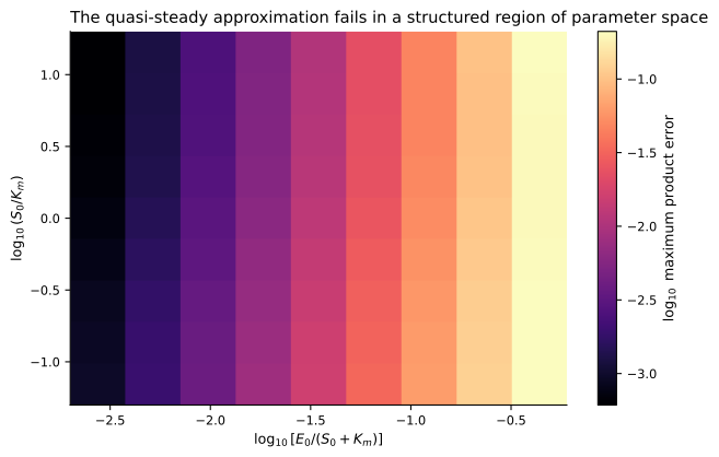
The poor corner has abundant enzyme relative to available substrate and low substrate saturation. The complex-formation transient is then not negligible compared with the overall conversion process.
A heat map forces a more careful statement than “Michaelis-Menten is valid when enzyme is small.” It reveals a graded surface, dependent on other ratios and on the metric used to colour it.
Is small (\varepsilon) sufficient?
The classical small-parameter condition
is informative. The atlas confirms that error generally decreases as (\varepsilon) decreases. It does not support a context-free cutoff.
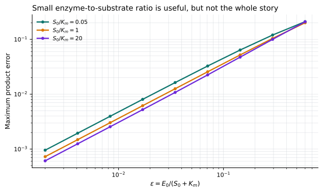
An approximation decision has at least four components:
- regime: which parameter ratios are plausible;
- quantity: product, substrate, complex concentration, or event time;
- horizon: early transient, depletion period, or late conversion;
- tolerance: what error changes the scientific or engineering decision.
The atlas records maximum and RMS product errors, substrate error, complex error, and relative errors in times to 50% and 90% conversion. No single number dominates every use case.
The initial layer is where the stories diverge
The full system begins with (C(0)=0). It must bind enzyme and substrate before appreciable product is formed. The QSSA trajectory begins directly on the algebraic relation
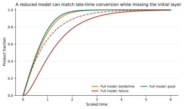
This has an inference consequence. If observations begin after the transient, a reduced model may fit product data while misrepresenting early complex dynamics. Good predictive fit on a restricted window does not prove that the eliminated mechanism was negligible at all times.
Conversely, an early mismatch need not make the reduction useless if the decision concerns only late conversion and the resulting error remains below tolerance. Validity is task-relative, not an all-or-nothing property.
Timing can fail before shape looks alarming
Suppose the model is used to set a sampling schedule, dosing interval, or residence time. Then an event-time error may matter more than a trajectory norm.
Define the relative half-conversion error
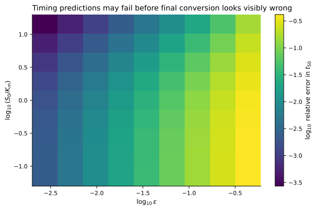
This is a general lesson for model reduction. Error should be measured on the quantity that drives the decision. A small (L^2) trajectory error does not guarantee a small threshold-crossing error, peak-time error, or control-action error.
The geometric reason QSSA works
In scaled variables, the QSSA relation is
It is an attracting lower-dimensional relation—a slow manifold approximation. The full trajectory first moves rapidly toward this relation and then travels slowly along it as substrate is depleted.
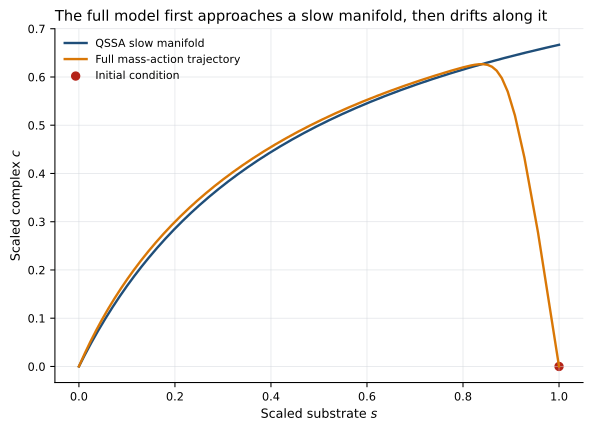
This picture is more useful than saying the complex is “constant.” It is not literally constant over the reaction. It adjusts rapidly to a moving relation determined by the slowly changing substrate.
For small (\varepsilon), attraction to the manifold is fast relative to depletion. For large (\varepsilon), the transient and slow phase overlap, so replacing the full path with motion constrained to the manifold becomes inaccurate.
What was verified
The full model is integrated with an implicit Radau solver because small-(\varepsilon) cases are stiff. The reduced equation is integrated independently, and both solutions are sampled on the same scaled time grid before metrics are calculated.
Three automated tests passed in the project’s pinned Python 3.12 and SciPy 1.16 environment. They verify conservation of total substrate,
monotone substrate loss in the reduced model, and lower QSSA error at a small (\varepsilon) than at a large comparison value. All 21 generated outputs passed checksum validation.
The atlas has no Monte Carlo uncertainty because both systems are deterministic. Its uncertainty is structural: parameter coverage, error definition, numerical tolerance, and omitted chemistry.
What the atlas does not establish
The mechanism assumes one substrate, one intermediate complex, irreversible product formation, perfect mixing, and constant rate coefficients. It omits:
- product and substrate inhibition;
- enzyme inactivation;
- cooperative or allosteric binding;
- multiple complexes or competing substrates;
- spatial diffusion and transport;
- stochastic effects at low molecular counts;
- parameter-estimation uncertainty.
The worst tested point is not a universal worst case. It is the worst among the declared grid. Extending the range or changing initial conditions and outputs can move the failure region.
The study also evaluates the standard QSSA only. Total QSSA and reverse QSSA can be preferable in other regimes. A model-selection workflow should compare reductions rather than force one approximation everywhere.
Turning the atlas into a decision tool
A useful next implementation would accept:
- plausible parameter ranges or posterior samples;
- an output such as (P(t)), (t_{50}), peak complex, or fitted parameter;
- a time window;
- an error tolerance.
It would then return the probability that the reduction satisfies the declared tolerance, together with representative failure trajectories. An adaptive sampler could refine the validity boundary instead of spending equal computation in obviously safe and unsafe regions.
For inference, synthetic data generated by the full model could be fitted with the QSSA model. That would reveal not only prediction error but parameter bias: a reduced model can fit observations by distorting (V_{\max}) or (K_m).
The main lesson is broader than enzyme kinetics: a reduced model is valid relative to a task, not by reputation. Michaelis-Menten kinetics is powerful precisely because it compresses a fast-slow mechanism. That compression should be tested where it will be used.
References
- Michaelis, L., & Menten, M. L. (1913). Die Kinetik der Invertinwirkung. Biochemische Zeitschrift, 49, 333–369.
- Johnson, K. A., & Goody, R. S. (2011). The original Michaelis constant: Translation of the 1913 Michaelis-Menten paper. Biochemistry, 50, 8264–8269. https://doi.org/10.1021/bi201284u
- Segel, L. A., & Slemrod, M. (1989). The quasi-steady-state assumption: A case study in perturbation. SIAM Review, 31, 446–477. https://doi.org/10.1137/1031091
- Segel, L. A., & Edelstein-Keshet, L. (2013). A Primer on Mathematical Models in Biology. SIAM.