When One Reactor Has Three Temperatures

A reactor can receive the same feed, use the same residence time, and face the same coolant condition, yet settle at more than one temperature. The statement sounds contradictory only if we expect a nonlinear system to have a single response to every input.

An exothermic continuously stirred-tank reactor creates a feedback loop. A warmer mixture reacts faster; faster reaction releases more heat; the released heat raises the temperature again. Heat removal opposes that loop, but the two mechanisms do not have the same shape. Their intersections can produce a cold stable state, a hot stable state, and an unstable state between them.

This study asks a more operational question than “how many roots does the steady-state equation have?” It asks which roots are reachable, why warming and cooling follow different paths, how a disturbance can move the reactor into another basin, and whether slow recovery reveals proximity to ignition.

The experiment is dimensionless and synthetic. It demonstrates mechanism and numerical workflow; it is not a safety calculation for a named plant.

A two-state heat–reaction model

Let (x) be the dimensionless concentration of unreacted material and (T) the dimensionless reactor temperature. The model is

\frac{dx}{dt}=1-x-k(T)x,

\frac{dT}{dt} =\varepsilon_T\left[T_f-T+B\,k(T)x-h(T-T_c)\right],

with an Arrhenius-like temperature response

k(T)=\mathrm{Da}\,e^{\gamma T}.

The concentration equation balances feed replacement against reaction. The temperature equation balances feed enthalpy, reaction heat, and heat transfer to coolant temperature (T_c). The default parameters are

\mathrm{Da}=1,\quad \gamma=2,\quad B=8,\quad h=1,\quad \varepsilon_T=0.1,\quad T_f=0.

They were selected to expose the nonlinear geometry clearly. They are not fitted kinetic or heat-transfer coefficients.

At equilibrium,

x^*(T)=\frac{1}{1+k(T)}.

Substitution into the energy balance gives a parametric description of the entire equilibrium branch:

T_c(T)= \frac{(1+h)T-T_f-B\,k(T)/(1+k(T))}{h}.

This is preferable to repeatedly asking a nonlinear root solver for one solution. A local solver can return whichever root is closest to its starting guess and conceal the other operating states. Parameterising the branch makes every candidate equilibrium visible.

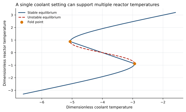
S-shaped equilibrium temperature branch with stable cold and hot segments, an unstable middle segment, and two folds. — **Figure 1.** The verified branch folds at coolant values \(-5.06568\) and \(-2.93432\). Between them, one input supports three equilibria, but the middle branch is unstable.

Three equilibria do not mean three operating choices

Stability is determined from the Jacobian

J= \begin{pmatrix} -1-k(T) & -xk'(T)\\ \varepsilon_T Bk(T) & \varepsilon_T\left[Bxk'(T)-(1+h)\right] \end{pmatrix}.

An equilibrium is locally stable when both eigenvalues have negative real parts. The outer cold and hot segments satisfy that condition; the intermediate segment does not. A small perturbation from the middle state grows until the trajectory falls into a stable basin.

This distinction changes the meaning of a steady-state diagram. Three algebraic roots are not three equally usable set-points. The unstable root is better understood as part of the boundary separating two long-term outcomes.

At a fold, a stable and an unstable equilibrium collide. The branch being followed simply ends. Once that happens, no amount of “slow control” can keep the system on the vanished state.

Why warming and cooling disagree

The continuation experiment begins on the cold branch and changes the coolant in small steps. At each step, the previous settled state initializes the next simulation. A second sweep begins on the hot branch and reverses the direction.

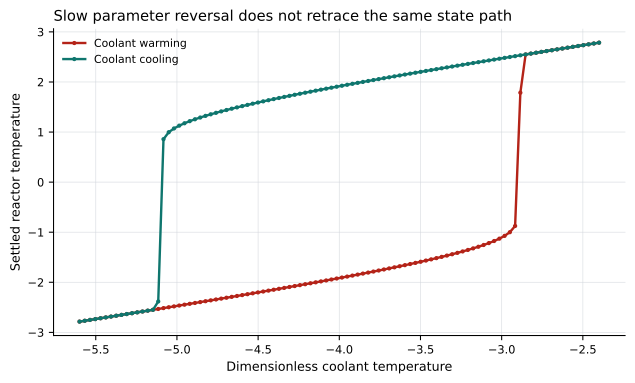
Warming and cooling continuation paths following different branches before abrupt ignition and extinction. — **Figure 2.** The cold state survives until the upper fold and then ignites; the hot state survives on the return journey until the lower fold and then extinguishes. The input–state relation therefore has memory.

The warming sweep jumps near (T_c=-2.885), close to the analytically located cold-branch fold at (-2.93432). The cooling sweep jumps near (T_c=-5.115), close to the hot-branch fold at (-5.06568). The small offsets are expected because each finite simulation must relax and because the continuation grid is discrete.

Hysteresis here is deterministic. No random shock is required. Two reactors at the same coolant setting can have different temperatures because their histories placed them in different basins.

That is the first practical lesson: input measurements alone may not identify the internal state. An operating record—whether the system approached from the cold or hot side—contains information that a static lookup table omits.

A dynamic coolant cycle

A quasistatic sweep pauses for relaxation. A real controller changes continuously. The next experiment therefore drives the coolant through a triangular cycle: warming at a constant rate and then cooling at the same rate.

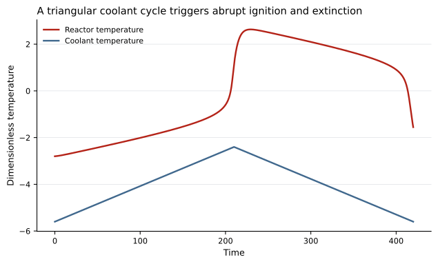
Triangular coolant cycle and reactor temperature trajectory with delayed ignition and extinction jumps. — **Figure 3.** Reactor temperature changes smoothly for long intervals and then jumps. The verified run reached a maximum dimensionless temperature of \(2.6317\), from an initial cold state near \(-2.8\).

The trajectory does not lie exactly on the equilibrium curve. Near a fold, relaxation slows while the control parameter is still moving. The observed transition can therefore lag the static bifurcation. Ramp rate, thermal time scale, and distance to the fold all matter.

This difference between a static safety envelope and a dynamic transition is easy to miss. A branch diagram explains what equilibria exist; a time-dependent simulation explains whether the system can track them under a particular control schedule.

Returning the input is not the same as restoring the state

Choose (T_c=-4), inside the multiplicity interval. Start the model from a grid of concentration–temperature pairs and integrate each point until it approaches either the cold or hot attractor.

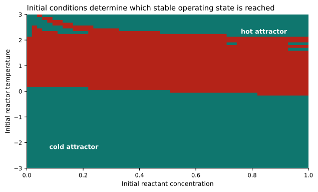
Initial concentration and temperature map divided into cold and hot basins of attraction. — **Figure 4.** The same external setting produces two stable outcomes. The unstable equilibrium and its stable manifold organise the basin boundary.

This provides a precise version of path dependence. A disturbance can cross the basin boundary without permanently changing the coolant. After the disturbance ends, restoring the old input may leave the reactor on the other stable branch.

The basin map is not a plant operating chart: it assumes perfect mixing and exact parameters. Its value is conceptual and diagnostic. It tells us what additional analysis becomes necessary in a calibrated study—uncertain basin boundaries, reachable disturbances, sensor coverage, and control actions that guarantee return rather than merely restore an input.

Recovery time as a proximity signal

Suppose a stable equilibrium is perturbed slightly. Linearisation gives

\dot{\delta z}=J\,\delta z.

If (\lambda_{\max}) is the eigenvalue with largest real part, a characteristic recovery time is

\tau_{\mathrm{rec}} \approx-\frac{1}{\operatorname{Re}(\lambda_{\max})}.

As the cold branch approaches its saddle-node fold, (\operatorname{Re}(\lambda_{\max})) approaches zero from below. The system remains stable, but it becomes less able to erase perturbations quickly.

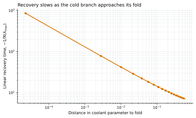
Linear recovery time increasing as the cold equilibrium approaches the ignition fold. — **Figure 5.** The rise in recovery time is a mechanistic consequence of the fold. It motivates perturbation-response monitoring, but it is not by itself a validated industrial alarm.

Absolute temperature can remain inside a familiar band while dynamic resilience is deteriorating. Recovery rate offers different information: how strongly the state is pulled back after a small deviation.

Critical slowing is not a universal detector. Measurement delay, coloured noise, unobserved states, drifting parameters, and feedback control can obscure or imitate it. A credible warning system would estimate recovery uncertainty, compare several indicators, and validate false-alarm performance on representative disturbances.

What was actually verified

The project does more than draw an S-curve. It parameterises the branch, classifies stability from Jacobian eigenvalues, integrates stiff trajectories with a Radau solver, performs warm and cold continuation, maps (55\times55) initial conditions, and calculates recovery time along the stable branch.

Three automated tests passed. They check that points on the parameterised branch satisfy the equilibrium equations, that the branch contains two folds, and that representative cold and hot equilibria are stable. The generated-output manifest contains 23 files and every checksum was revalidated. The numerical claims in this article come from that default run.

These checks establish internal reproducibility. They do not validate the model against an experiment, identify an industrial safety margin, or prove that an early-warning statistic will work under plant noise.

A useful next study

The most valuable extension is not simply a more elaborate reaction network. It is an uncertainty-aware control study built around the fold geometry:

calibrate kinetics and heat transfer to experimental data;
continue equilibria with pseudo-arclength methods and test for Hopf bifurcations;
propagate parameter uncertainty into fold and basin locations;
impose sensor delay, actuator saturation, and coolant disturbances;
compare temperature thresholds with recovery-based alarms;
design a controller that respects probabilistic distance from the unsafe transition.

That workflow preserves the central insight of the simple model while asking questions a real decision system must answer.

The main lesson is therefore not that nonlinear equations sometimes have three roots. It is that stability, history, and recovery determine which root matters. A reactor can appear steady, remain far from its other stable state, and still be moving toward a point where its present operating branch ceases to exist.

References

Chidambaram, M. (2018). Mathematical Modelling and Simulation in Chemical Engineering. Cambridge University Press. https://doi.org/10.1017/9781108672887
Aris, R. (1965). Introduction to the Analysis of Chemical Reactors. Prentice-Hall.
Strogatz, S. H. (2015). Nonlinear Dynamics and Chaos (2nd ed.). Westview Press.
Berezowski, M. (1994). Continuous reactions in a non-isothermal CSTR—I. Multiplicity of steady states. Chemical Engineering Science, 49, 1789–1799. https://doi.org/10.1016/0009-2509(94)85008-9