
A pressure sensor is useful only while its measurement reaches the model. That sounds obvious, but it changes how a monitoring network should be designed.
Suppose a water utility can install seven sensors. A conventional placement method may spread them so that the complete seven-dimensional pressure signature distinguishes many possible leaks. During maintenance, packet loss, calibration rejection, or a power interruption, one coordinate disappears. If that coordinate carried the only useful difference between two leak zones, the nominally strong layout becomes ambiguous.
This project asks a narrower question than “can we detect every real leak?” It asks whether a sensor layout can preserve the shape of diagnostic evidence after any one selected sensor is removed. The current result is a synthetic pilot, designed to expose the method and its failure modes before attempting a claim about an operational network.
Research question and claim boundary
The research question is:
Can pressure sensors selected for lower-tail leak-signature separation retain localisation performance when measurements are noisy and one sensor may fail?
This wording fixes three things before looking at the result. First, the task is localisation: choosing among candidate leak zones, not detecting an unknown leak onset. Second, the failure model removes one pressure sensor, not an arbitrary part of the network. Third, the evidence comes from controlled signatures, not field pressure data.
The study is therefore deliberately narrow. It consists of:
- a scale-invariant way to measure how distinguishable candidate leak signatures are;
- a placement objective that tests every possible one-sensor removal;
- a greedy algorithm that can be inspected without a black-box optimiser;
- a paired Monte Carlo benchmark against random, degree-based, and nominal greedy layouts;
- reporting that includes aggregate, top-3, and worst-zone performance.
The study does not claim a new hydraulic solver, real-time deployment, or validation on a named city. Its current status is synthetic benchmark only—useful for comparing placement ideas, not for claiming field performance.
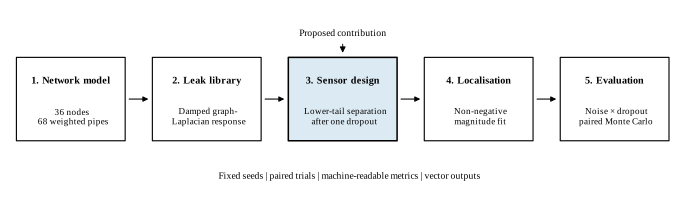
The complete evidence pipeline. Only the highlighted placement stage is proposed; the surrounding stages make its assumptions and evaluation auditable.
Turning a pipe network into diagnostic signatures
The experiment uses a 36-node meshed graph. One node is a fixed-head reservoir; the other 35 are candidate leak zones. Conductance-weighted edges represent pipes. A damped graph Laplacian gives a pressure-response proxy for a unit leak at each candidate node:
Here, is the reduced conductance Laplacian, injects a leak disturbance at node , and is a small damping term. The resulting column is not a full hydraulic simulation. It is a controlled way to create smooth, topology-dependent pressure signatures and test the placement logic.
That distinction matters. EPANET can represent nonlinear head loss, pumps, valves, tanks, time-varying demand, and pressure-dependent behaviour. This pilot represents none of those in full. A graph proxy makes the algorithm easy to inspect; it does not make the output a field result.
What the proxy preserves
Although simplified, the proxy preserves several structures needed for a placement experiment:
- disturbances propagate through connected pipes rather than independently at each node;
- conductance changes the strength of that propagation;
- nearby leak zones can have similar pressure signatures;
- sensors at different locations observe different projections of the same disturbance;
- the fixed-head reservoir anchors the otherwise singular graph Laplacian.
Each full signature is divided by its maximum absolute response before placement. During classification, the leak magnitude is fitted again. This separates the spatial pattern of a response from its absolute scale. The choice is useful when leak magnitude is uncertain, but it also removes information that a calibrated hydraulic model might legitimately use.
What the proxy omits
The model does not contain elevation, pipe diameter, Hazen–Williams or Darcy–Weisbach head loss, pumps, valves, tanks, demand schedules, or pressure-dependent demand. It assumes one leak at a time and represents a leak as an added nodal demand. The damping term stabilises the response but has not been calibrated to a physical network.
These omissions are not hidden implementation details. They define the boundary of the result. The current experiment tests whether dropout-aware geometry is promising enough to justify a more expensive hydraulic study.
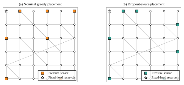
The nominal greedy layout optimises intact-system signature separation. The proposed layout changes that selection by scoring the evidence left after each possible one-sensor dropout.
Placing sensors for the incomplete observation
For a proposed sensor set , the model restricts every leak signature to those sensor locations. It then removes each sensor in turn, normalises the remaining signatures, and measures pairwise distance:
The fifth percentile focuses on difficult pairs without letting one almost-identical pair control every decision. Taking the minimum over possible dropouts asks the layout to retain separation whichever single sensor disappears. A greedy search adds the candidate that improves this score most.
In pseudocode, the placement stage is:
S ← empty sensor set
while |S| < sensor budget:
    for each candidate c not in S:
        T ← S ∪ {c}
        for each possible failed sensor d in T:
            restrict every leak signature to T \ {d}
            normalise each restricted signature
            compute all pairwise distances
            score dropout d by the 5th percentile distance
        score candidate c by the worst dropout score
    add the highest-scoring candidate to S
return S
This is not globally optimal. Forward selection can commit early to a sensor that later prevents a better combination. Its advantages are transparency, deterministic output, and a direct link between the objective and the selected locations. A more thorough comparison would include exhaustive search on small networks and stronger combinatorial or population-based methods on larger networks.
Three comparisons keep the proposal honest:
- a fixed-seed random layout;
- the seven highest-degree nodes;
- a nominal greedy ablation that uses signature separation but never removes a sensor while scoring the layout.
The third comparison is the important one. If dropout-aware placement only beats random or degree centrality, the gain might come from using signature information at all. Beating the nominal ablation under sensor loss is the more specific test of the research idea.
The degree baseline is also informative for a different reason. Highly connected nodes look important from topology alone, yet diagnostic value depends on how differently candidate leaks affect the sensors. Centrality and identifiability are not the same objective.
A deliberately stressed benchmark
Each simulated observation varies leak magnitude uniformly from 0.65 to 1.35. Gaussian noise is scaled relative to the active leak signature. With a configured probability, one of the seven sensors is removed. The classifier fits a non-negative magnitude for every candidate leak and chooses the template with the smallest residual.
The experiment crosses five noise levels—2%, 5%, 8%, 12%, and 16%—with dropout probabilities of 0%, 20%, and 40%. Every method-condition pair covers all 35 leak zones with 35 trials per zone: 1,225 trials. Common random seeds are used across methods at each condition so that layouts see the same sequence of leak magnitudes, noise, and dropout decisions.
| Design element | Setting |
|---|---|
| Network | 36 nodes, 68 weighted pipes, one fixed-head reservoir |
| Candidate leak zones | 35 |
| Sensor budget | 7 |
| Placement methods | Random, degree, nominal greedy, dropout-aware greedy |
| Relative noise | 2%, 5%, 8%, 12%, 16% |
| One-sensor dropout probability | 0%, 20%, 40% |
| Leak magnitude multiplier | Uniform from 0.65 to 1.35 |
| Trials per condition | 35 zones × 35 repeats = 1,225 |
| Primary metrics | Top-1, top-3, worst-zone top-1 |
| Uncertainty display | Wilson 95% interval for aggregate top-1 proportion |
For an observation and candidate template , the classifier estimates a non-negative leak magnitude,
and ranks candidates by the residual . This is a small, interpretable inverse problem. It avoids training a classifier whose capacity could obscure whether gains come from placement or prediction.
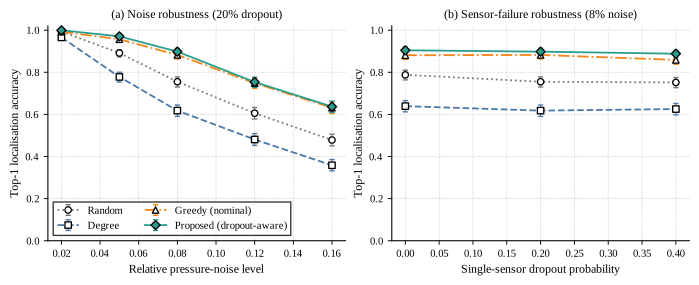
Top-1 localisation accuracy across the experiment matrix. Error bars are Wilson 95% intervals for aggregate proportions; they do not capture every within-zone dependence.
What the result supports
At the designated stress condition—8% relative noise and a 40% probability of losing one sensor—the dropout-aware layout achieved 88.8% top-1 accuracy. The nominal greedy layout achieved 85.9%, random placement 75.2%, and degree placement 62.5%. Top-3 accuracy for the proposed layout was 98.3%.
| Placement | Top-1 | Wilson 95% interval | Top-3 | Worst-zone top-1 |
|---|---|---|---|---|
| Random | 75.2% | 72.7–77.5% | 95.1% | 22.9% |
| Degree | 62.5% | 59.8–65.2% | 87.8% | 20.0% |
| Nominal greedy | 85.9% | 83.8–87.7% | 97.9% | 51.4% |
| Dropout-aware greedy | 88.8% | 86.9–90.5% | 98.3% | 65.7% |
The proposed-versus-nominal top-1 difference is 2.9 percentage points in this condition. Because both methods were evaluated with common random numbers, this is a paired experimental design. The displayed Wilson intervals describe each aggregate proportion separately; they are not a formal confidence interval for the paired difference. The article therefore reports an observed improvement, not statistical superiority.
The worst-zone result is more revealing. Aggregate accuracy can hide a neighbourhood whose leak signatures are repeatedly confused. The proposed layout’s least accurate zone reached 65.7%, compared with 51.4% for the nominal ablation, 22.9% for random, and 20.0% for degree placement.
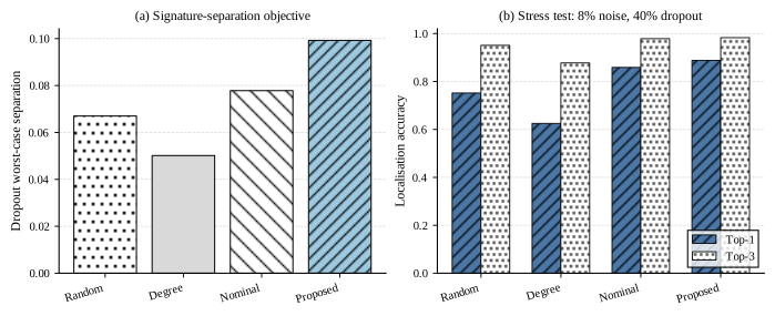
The proposed layout improves the dropout-aware separation objective and the selected stress test, but this does not establish universal dominance.
The result is promising, but it is not uniform. At 12% noise and 40% dropout, aggregate top-1 accuracy was 73.7% for the proposed method and 74.0% for nominal greedy—effectively level. At 16% noise the proposed method recovered an aggregate advantage, yet its worst-zone score fell below nominal. A placement objective built around lower-tail geometric separation does not automatically optimise every fairness or extreme-noise metric.
Reading the robustness curves
The left panel of the robustness figure fixes dropout probability at 20% and increases measurement noise. All four methods deteriorate, as expected. The meaningful comparison is not whether accuracy falls, but whether a placement retains a useful margin over baselines as signatures become harder to distinguish.
The right panel fixes noise at 8% and increases the probability that one sensor is missing. This is closest to the placement objective. The proposed layout is designed for the consequence of losing a sensor, not simply the probability of failure. A 40% dropout probability does not mean 40% of sensors disappear; it means that in 40% of trials, exactly one of the seven measurements is unavailable.
The top-3 result adds operational context. When top-1 localisation is wrong, a high top-3 score means the true zone is often still in a small inspection shortlist. That may matter for staged diagnosis, but it is not equivalent to an automatic correct localisation. The utility of top-3 depends on the cost of inspecting several zones.
Why the proposed layout may help
The topology figure shows that the robust objective does more than add a post-processing rule to the same layout. The nominal and dropout-aware methods retain some common sites but reassign others because a coordinate that is valuable in the intact signature matrix may also be a single point of diagnostic dependence. The figure does not prove why each site was selected; the separation objective and ablation provide that evidence.
This interpretation is consistent with the objective, but it is not causal proof. A larger experiment should quantify spatial diversity, signature redundancy, and the frequency with which each failed sensor changes the predicted zone. That analysis would show whether the gain is genuinely caused by dropout redundancy or by another geometric property of the selected set.
Validity threats
A careful account is stronger when it states how it could be wrong.
Construct validity
The fifth-percentile signature distance is a proxy for diagnostic usefulness. It does not directly optimise top-1 accuracy, response time, repair cost, or equitable service impact. The worst-zone metric partly addresses this gap, but future work should connect placement to operational loss.
Internal validity
The implementation uses fixed seeds and common random numbers, and unit tests check matrix shape, clean-signature identification, and unique sensor selection. These controls reduce accidental variation. They do not rule out a modelling bug, a poorly chosen stress condition, or sensitivity to the fixed random baseline.
External validity
One synthetic network cannot establish performance on tree-like, highly looped, pressure-deficient, or operationally controlled water networks. The experiment includes no demand pattern, pipe uncertainty, elevation, or field sensor behaviour. Generalisation remains untested.
Statistical conclusion validity
There are 1,225 trials per method-condition pair, but trials share leak zones and network structure. Aggregate binomial intervals do not model every dependence. A stronger analysis should retain paired trial outcomes, report paired bootstrap intervals, repeat random layouts, and pre-register one or more primary conditions before comparison.
Reproducing the study
The calculation can be regenerated without a notebook. From the project directory:
python -m venv .venv
.venv/Scripts/python -m pip install -r requirements.txt
.venv/Scripts/python run.py
.venv/Scripts/python -m unittest discover -s tests -v
On macOS or Linux, replace .venv/Scripts/python with .venv/bin/python. The experiment writes:
- a complete 60-row condition table to
results/benchmark_metrics.csv; - selected sensor nodes and the designated stress test to
results/summary.json; - four reviewed vector figures to
figures/publish/; - no article prose.
The last point is intentional. A rerun can update evidence and figures, but it cannot silently rewrite the interpretation.
Why keep the article separate from the calculations
The ScienceProject directory holds the evidence: source code, generated metrics, test record, paper draft, and approved figures. This article interprets a selected result and explains its limitations. Running the experiment can update the evidence and figures, but it cannot overwrite this prose.
That separation is part of the research method. Computation should make a claim auditable; editorial review should decide whether the claim deserves to be public.
Conclusion
The synthetic pilot supports one careful conclusion: explicitly representing a missing pressure sensor changes the selected layout and improves the designated stress-case result over a nominal signature-based ablation. The observed gain is modest in aggregate top-1 accuracy and larger for the least accurate leak zone. It is not uniform under every noise setting.
That is enough to motivate a follow-up study, but not enough to justify deployment language. The value here is the chain from a narrow question to reproducible evidence, an ablation, limitations, and a written plan for what would need to change before the result could leave the benchmark.
Technical sources
- U.S. Environmental Protection Agency, EPANET 2.2 and its hydraulic modelling documentation.
- M. V. Casillas et al., “Pressure Sensor Placement for Leak Localization in Water Distribution Networks Using Information Theory”, Sensors, 2022.
- M. K. Hasan et al., “A Two-Stage Model for Data-Driven Leakage Detection and Localization in Water Distribution Networks”, Water, 2023.
These sources position the problem. The numerical claims in this article come only from the linked ScienceProject experiment and its generated metric table.