Topology at the Edge of Resolution: Which Melt-Pond Signals Survive the Camera?

Summer sea ice can look almost binary from above: dark water between brighter snow and ice. Yet the apparent network is partly made by the camera. Blur can erase an ice bridge; downsampling can invent a water channel; a classifier can join ponds by moving one observed pixel; and cropping can turn a local cluster into an edge-to-edge crossing.

Connectivity is discontinuous: a few pixels can merge components, close a loop, or create the first spanning path. Area changes gradually; topology can jump. Any study using that jump as a percolation signal must include resolution and segmentation in its mathematical model.

This study asks a deliberately measurement-focused question:

If a high-resolution latent melt-pond pattern has a well-defined connectivity transition, which image diagnostic still locates that transition after realistic observation errors have altered the pattern?

Six diagnostic families receive the same latent patterns, degraded views, truth, and failure accounting: direct spanning, pond fraction, an area–perimeter breakpoint, Euler/Betti curves, persistence-pruned Betti curves, and a pond-interior distance bottleneck. Resolution-robust means passing predeclared error and failure limits in every held-out morphology and stress stratum.

This computational benchmark, with a bounded observational case, neither infers an Arctic-wide threshold nor reconstructs subsurface hydraulics. Synthetic fields provide known truth; MOSAiC shows how to audit real imagery without treating segmentation as nature itself.

Explore the measurement problem first

The compact laboratory below is not the evidence engine. It is a teaching-scale model designed to make the discontinuity visible. Choose a synthetic morphology, move the water level, then reduce the effective resolution or add boundary error. Watch the pond fraction change smoothly while component counts, loops, and edge-to-edge spanning can change in a single step.

Try to construct two images with almost the same pond fraction but opposite spanning decisions. Then keep the latent field fixed and alter only blur. This is the core identification strategy of the research: paired observations isolate the effect of the camera and classifier from the effect of the underlying morphology. The full Melt-Pond Topology Lab adds direction-specific spanning, connectivity conventions, and more diagnostic curves.

Why connectivity matters, and why area is not enough

Melt-pond coverage enters sea-ice albedo and energy calculations, while geometry affects lateral melt, transmitted light, drainage, and connectivity. Nicolaus and colleagues establish the qualitative light connection; no corrected irradiance value is used here. Polashenski, Perovich, and Courville documented staged controls from supply, topography, permeability, and drainage, and a later Polashenski-led study demonstrated freshwater-driven percolation blockage. Similar dark-pixel fractions can therefore represent different physics.

Pond fraction is nevertheless a scalar. Let a binary mask on a domain $D$ be $M(x,y)\in\{0,1\}$, with one denoting pond water. Its coverage is

or the water-labelled pixel proportion. It says nothing about arrangement: compact ponds, a lace-like network, and one stripe can share $\phi$, although only the stripe must span. Coverage cannot simultaneously be geometry, topology, and threshold detector.

Hohenegger and colleagues found an area–perimeter transition from simple small-pond boundaries toward complex large ones; it was not a direct connectivity test. Popović and colleagues reproduced multiple statistics with an overlapping-circle void model resembling near-percolation clusters. Ma and colleagues reproduced scaling and fractal-transition behaviour with a random-field Ising model. These studies motivate threshold language while distinguishing its observables.

A fractal-dimension breakpoint need not equal first finite-window spanning; time, pond fraction, and minimum traversable width also index different events. Rather than choose one published threshold as “correct,” the benchmark measures how each operational definition moves under a controlled observation process.

Topology in a pixel image

Topology ignores exact lengths and angles and asks what remains connected under continuous deformation. For a two-dimensional pond mask, the first two Betti numbers supply a compact vocabulary:

The Euler characteristic is

As water rises, isolated depressions merge and $\beta_0$ falls; channels around ice islands can raise $\beta_1$, before flooding closes loops. These events need not coincide with first spanning, but their curves reveal reorganisation hidden by area fraction.

Digital topology needs a corner convention: treating both phases symmetrically at diagonals can let each pass through the same corner. The primary model uses pond four-connectivity and ice eight-connectivity; the reverse is an ablation. Horizontal and vertical spanning remain separate because anisotropic patterns may cross one direction first.

Spanning is defined on a finite square rather than an infinite lattice. Let $S_x(M)=1$ if at least one pond component touches both the left and right boundaries, and let $S_y(M)=1$ for top-to-bottom connection. The benchmark reports

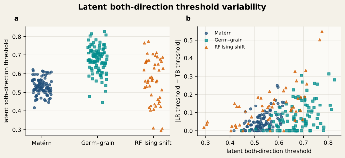
For nested filtration $M(u)$, the horizontal threshold is the first level with $S_x=1$. We map generator-specific score units to latent pond fraction:

Vertical, any-, and both-direction definitions follow. The primary target is latent first both-direction spanning before observation error; the other thresholds are supporting diagnostics.

Persistent homology adds scale, not immunity

Single-threshold Betti counts give short-lived features full weight. Persistent homology follows each feature from birth $b$ to death $d$, with lifetime $|d-b|$; near-diagonal diagram points are short-lived.

The positive pond-interior branch of a Euclidean distance transform assigns each water pixel its distance to ice, so thresholding it asks which channels retain a minimum radius. Robins and colleagues linked signed-distance persistence to percolating scales in porous media; Offord and colleagues adapted it to melt-pond models. Here the constructions remain separate: exact elder-rule $H_0$ and dual $H_1$ bars come from the scalar pond-score field, while the throat statistic is a direction-specific maximum-bottleneck path on positive pond-interior distance. It creates no distance-transform persistence bars.

Persistent homology has already been applied to melt ponds, and SEDT persistence to percolation. The contribution is instead a paired stability comparison across pixel size, blur, segmentation displacement, boundary error, and crop, including whether pruning suppresses false transitions without deleting a genuine thin channel.

Edelsbrunner, Letscher, and Zomorodian formalised feature lifetime and simplification within a filtration. Cohen-Steiner, Edelsbrunner, and Harer then proved, under suitable regularity, that a bounded filtering-function perturbation bounds bottleneck displacement. This does not make every downstream threshold stable: downsampling can delete features, hard segmentation is discontinuous, cropping changes the domain, and selecting one feature or sign change can amplify a small movement. Stability therefore remains a tested hypothesis.

The measurement gap left by the literature

Field work links pond evolution to supply, topography, permeability, and drainage; geometry and statistical physics identify scaling and coalescence; topology measures components, loops, throats, and spanning. Miao and colleagues combined spectral, textural, and spatial relationships for object-based remote-sensing classes, while Niehaus and colleagues estimated fractional ponds in Sentinel-2 pixels. These strands establish relevance, not invariance to raster construction.

A fractional 10 m pixel, object polygon, and 0.5 m binary cell are different mathematical objects. Equal coverage does not guarantee adjacency, nor does area uncertainty bound first-spanning error. The paired stress test and abstention gate measure that gap; any positive result would remain benchmark evidence, not sensor-independent Arctic criticality.

Three morphology families instead of one convenient world

A diagnostic can look robust when the generator happens to favour it. To reduce that danger, the benchmark separates development from held-out morphology shift.

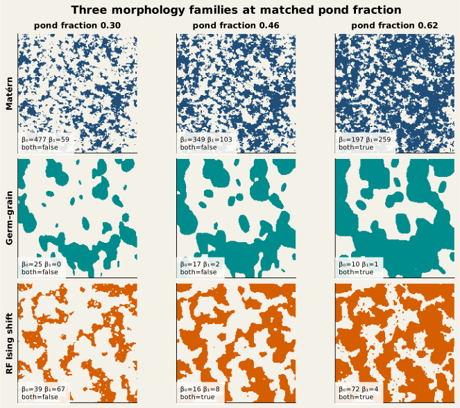
The first generator is an anisotropic Matérn Gaussian random field. A spectral construction produces a smooth latent pond-score field $Z(x,y)$, where higher values are more pond-like, with controllable correlation length, roughness, and directional anisotropy. Pond masks are superlevel sets,

Lowering $u$ makes the filtration exactly nested. Correlation controls the typical basin scale; anisotropy can create elongated channels and a gap between horizontal and vertical thresholds. This family is mathematically clean but not asserted to be a calibrated topography model for any particular floe.

The second generator is a Boolean germ–grain model. Random ellipses represent growing water regions or, in a complementary void formulation, ice obstacles. Their centres, sizes, aspect ratios, and orientations control coalescence. This family connects directly to the overlapping-object intuition in Popović and colleagues while allowing directional structure. Its boundaries can be sharper and its merging events more geometric than those of the Gaussian family.

The third generator is a random-field Ising morphology used only after the diagnostic definitions are frozen. Local interactions favour agreement between neighbouring water/ice states, while a spatial random field introduces heterogeneous preferences. The family draws on the statistical-physics perspective of Ma and colleagues, but the benchmark implementation is a controlled synthetic shift rather than a fit to their physical parameters. Holding it out tests whether a rule tuned on smooth fields and overlapping grains survives a different coarsening mechanism.

Each latent field is generated at $512\times512$ pixels for the main benchmark. A smaller exploratory sample is used to set algorithmic choices. A separate six-field audit, alternating Matérn and germ–grain realizations at $512^2$ and $1024^2$, checks whether selected latent thresholds are themselves discretisation artefacts; it is not a repeat of the full held-out experiment. Every realization has a fixed identifier plus deterministic generator parameters and seed under the recorded configuration hash. The article never selects a visually appealing field and treats it as a distribution.

The observation operator is part of the model

Let $Z$ denote a latent continuous-valued field or a distance-like representation of a latent mask. The observed image is constructed by a declared composition,

followed by segmentation

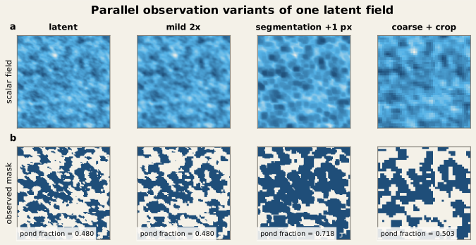
Here $K_\sigma$ is a Gaussian point-spread kernel; $\mathcal S_h$ is anti-aliased block sampling at effective pixel size $h$; $\varepsilon_r$ is radiometric noise; $\varepsilon_b$ is high-pass boundary-scale texture; $\mathcal B_\rho$ is a grayscale boundary-displacement operator; and $\mathcal C_W$ applies the final central crop. The declared positive-bias stratum uses $\rho=+1$: one observed-pixel grayscale dilation after exactly the same blur, downsampling, radiometric noise, and random stream as the mild stratum. At every threshold, its superlevel mask is therefore exactly the corresponding one-pixel binary dilation. It is not a global additive score offset. Every generator produces a scalar pond-score field, so this order is fixed and logged before thresholding.

Order matters. Thresholding before averaging answers whether most subpixels are water; averaging before thresholding answers whether the pixel’s mean response crosses a radiometric boundary. Eroding after downsampling is not equivalent to eroding before it. Cropping before connected-component labelling changes which features touch an edge. The evidence pipeline records per-stack outputs and retains one representative preview rather than archiving every intermediate mask; a separately tested identity setting must return the latent raster exactly.

The paired design reuses each latent field across all observation settings. Suppose one downsampling level produces a crossing and the next does not. Because the latent field is identical, this difference belongs to the observation operator rather than to morphology sampling. Bootstrap resampling occurs at the latent-field level so multiple degraded views of one field are never treated as independent evidence.

Six competing ways to call a transition

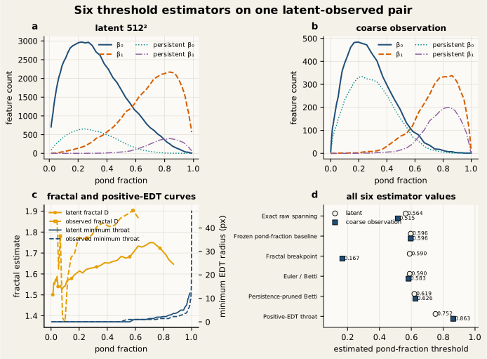
Direct observed spanning locates the first segmented mask that spans in both horizontal and vertical directions. It matches the primary target most closely, but is maximally exposed to a single bridge or break. Single-direction spanning remains a supporting audit.

Pond fraction alone always predicts one constant: the median latent threshold calibrated on discovery fields. It does not inspect each observed image stack. If a universal critical coverage existed across generators and directions, this deliberately information-poor baseline would be hard to beat. Poor performance would show why a coverage value learned in one morphology cannot automatically transfer to another.

The area–perimeter fractal breakpoint regresses log perimeter on log area across components at every filtration level using $P\propto A^{D/2}$, smooths the resulting dimension curve over pond fraction, and selects the largest absolute gradient. It connects with Hohenegger and colleagues without claiming a direct piecewise fit. Minimum component counts and smoothing are frozen; an unidentified breakpoint is counted as a failure.

Euler and Betti curves use the sampled zero crossing of $\chi=\beta_0-\beta_1$ over pond fraction, restricted to the frozen admissible coverage interval. If no sign change appears, the rule takes the sampled admissible point closest to zero. This is a fixed estimator, not a discovery-stage choice among several curve landmarks.

Persistence-pruned Betti curves count exact elder-rule $H_0$ and dual $H_1$ bars, remove bars with contrast lifetime below $0.18$, then apply the same Euler zero-crossing rule. Bars are evaluated on a deterministic strided grid capped at $96\times96$ for comparable cost. This internal compute grid is separate from simulated sensor resolution and can itself alias a narrow connection.

That cap is a computational sensitivity choice, not an observational claim. The stride is fixed before evaluation and reused across paired settings, so it cannot quietly adapt to a favourable image. The audit nevertheless treats disagreement between the capped topology calculation and the full latent raster as method error rather than sensor error.

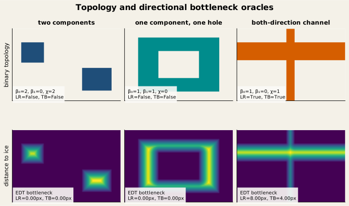
The pond-interior EDT maximum-bottleneck throat finds the first level at which positive-distance paths of radius at least 1.5 observed pixels span in both directions. It therefore rejects a crossing supported only by a thinner observed channel. The 1.5-pixel rule adds a frozen geometric scale to binary spanning, at the cost of extra computation and explicit dependence on observed pixel size.

No metric is allowed to redefine “truth” in its own image. The estimand is always error relative to the high-resolution latent spanning threshold expressed in latent pond fraction. That separation prevents a topological method from winning simply because truth was defined using the same topological statistic.

A frozen experiment rather than a figure hunt

The discovery stage contains 96 latent fields and 576 paired observation stacks. It is used to debug estimators, fix smoothing and breakpoint rules, set persistence pruning, and define how a missing threshold is recorded. The held-out stage contains 144 new latent fields and 864 paired stacks, including the unseen Ising family and named high-stress settings. The estimand, configuration, diagnostics, and decision gates are frozen before confirmatory v4. Figure presentation is corrected during audit without changing a metric or selection rule.

The primary error for field $i$ and diagnostic $d$ is

For each generator and stress stratum, median, 90th percentile, and root mean squared error are conditional on successful estimates. The proportions within $0.02$ and $0.05$ use every declared stack, with an unresolved estimate counted as a miss; failure rate is reported separately. Any-direction thresholds and the aggregate mean horizontal/vertical absolute error provide secondary directional audits. Runtime is retained because a multiscale diagnostic that is marginally more stable but much slower may be unsuitable for large image archives.

A method is called resolution-robust within this benchmark only if, in every declared held-out generator and stress stratum, its median absolute error is at most $0.02$, its 90th-percentile error is at most $0.05$, and its failure rate is at most five percent. These limits are not physical constants. They are a demanding, visible decision rule that prevents the article from describing the best of several weak methods as robust merely because it ranks first.

Uncertainty intervals use 2,000 generator-stratified paired bootstrap resamples of latent fields. All six observations derived from one field travel together in a resample. Comparisons between diagnostics are paired within field and stress setting. Denominators and missing thresholds remain explicit.

Verification before comparison

A complicated pipeline can produce polished but meaningless stress maps if its elementary topology is wrong. The first verification layer uses five tiny masks with exact answers: an empty mask, one and two isolated components, one ring, and a domain with two holes. Computed counts of $\beta_0$, $\beta_1$, and $\chi=\beta_0-\beta_1$ must match those hand-derived values.

The second layer cross-checks algorithms rather than adding more narrative examples. Exact elder-rule $H_0$ and dual $H_1$ curves must match direct binary Betti counts at sampled thresholds. The filtration must be nested, and an identity observation operator must preserve the scalar field bit for bit. The ordered-pixel spanning oracle must preserve occupied-fraction thresholds under a positive affine transformation of scalar scores; a separate 61/241/961/3841-level audit records convergence of the superseded sampled approximation.

The third layer uses known stochastic structure. Independent site occupation on a triangular lattice has critical probability one half in the infinite limit. Finite grids do not cross exactly at one half, so the test checks convergence and symmetry rather than forcing every realization to a textbook constant. It detects reversed inequalities, boundary mistakes, and a failure to distinguish finite-sample crossing probability from an asymptotic threshold.

The fourth layer targets multiscale geometry. A bounded scalar perturbation is checked through the two filtration inclusions implied by its sup norm; the code does not claim to solve a numerical diagram-matching problem in that check. A constructed dumbbell must recover its horizontal pond-interior EDT throat within one pixel and must not span vertically. A Sierpiński-carpet fixture checks the box-counting estimator against its known dimension. These checks validate implemented quantities; they do not prove that persistence or fractal geometry is the best threshold estimator.

Finally, a six-field latent convergence audit alternates Matérn and germ–grain realizations and compares their both-direction thresholds at $512^2$ and $1024^2$. It does not rerun all 864 observed stacks at the finer grid. Deterministic seeds, the frozen configuration hash, and a claim–evidence ledger connect public results to machine-readable outputs.

What survived the camera

The frozen evidence run compares all six diagnostic families without changing the gate after inspection. The answer is an abstention: none passed the median, tail-error, and failure limits in every generator-by-observation stratum. Raw spanning had the lowest pooled median absolute error, $0.0144$, with a 95% field-bootstrap interval of $[0.0124,0.0163]$, but its pooled 90th percentile was $0.0666$, above the $0.05$ gate. A favourable centre did not protect the tail.

Interpretation has three layers: latent variation across morphologies, movement under the declared observation operator, and recovery of the latent target. Ranking estimators without separating those layers can mistake shared observation bias for stability.

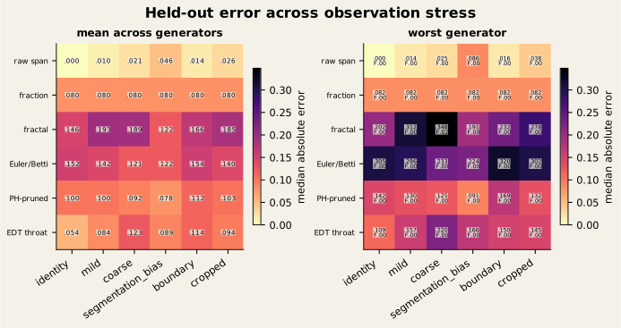
Figure 6 locates that failure. Under the paired one-pixel segmentation displacement, raw spanning on Matérn fields reached median error $0.08555$ and 90th-percentile error $0.12913$ across $48$ stacks; none fell within $0.02$, and only $10.42\%$ fell within $0.05$. Other diagnostics failed for different reasons: the worst conditional median was $0.3482$ for the fractal breakpoint on coarse Matérn observations, $0.3204$ for Euler/Betti on boundary-perturbed Ising fields, $0.1691$ for persistence-pruned Betti on that same stratum, and $0.2201$ for the EDT throat on coarse Matérn views. These are separate worst strata, not one composite scene.

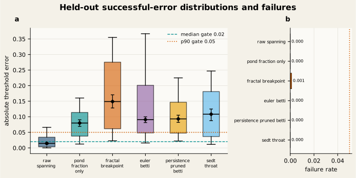
Across all $864$ held-out stacks, conditional median / 90th-percentile errors were $0.0144/0.0666$ for raw spanning, $0.0799/0.1603$ for pond fraction, $0.1489/0.3553$ for the fractal breakpoint, $0.0908/0.3696$ for Euler/Betti, $0.0931/0.2278$ for persistence-pruned Betti, and $0.1082/0.2470$ for the EDT throat. Fractions within $0.05$, using every stack, were respectively $84.03\%$, $30.56\%$, $21.06\%$, $26.50\%$, $25.93\%$, and $29.86\%$. The fractal estimator was unresolved once—one coarse Ising stack out of $864$; every other diagnostic resolved all $864$. Thus even the best pooled method cannot be promoted to a universal signal.

Where a method breaks is part of the result

Average error can conceal qualitatively different failure mechanisms. Direct spanning is vulnerable to a single bridge. Pond fraction ignores arrangement and can transfer a morphology-specific coverage threshold into the wrong generator. Fractal breakpoints can become unidentified when too few component scales survive downsampling. Betti curves can be dominated by pixel-scale components. Persistence pruning can delete a genuine narrow neck. The bottleneck throat can be stable in width yet fail to identify the first latent coverage at which any path appears.

The segmentation-displacement comparison is unusually well isolated: it differs from the paired mild view only by the one-pixel grayscale dilation. It is a separate stratum, not an operation silently combined with the coarse view. Paired rows retain latent any-direction, horizontal, and vertical thresholds, the observed any-direction threshold, and the aggregate mean horizontal/vertical absolute error, alongside primary both-direction absolute errors and failure rates. They do not retain separate observed horizontal and vertical series. Two strata with similar absolute error need not describe the same directional failure.

The benchmark therefore includes ablations for anisotropy, finite window size, generator shift, connectivity convention, persistence threshold, and the $512^2$ versus $1024^2$ latent grid. Latent horizontal and vertical thresholds are inspected separately to expose anisotropy; observed directional error follows the declared aggregate mean of horizontal and vertical absolute errors. Any method that succeeds only on nearly isotropic fields is described that way.

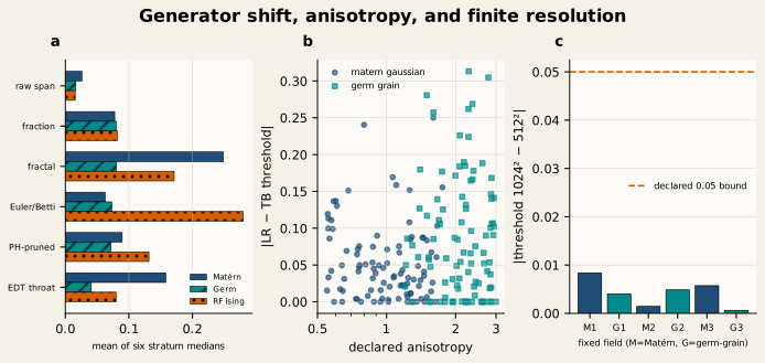
All fourteen named numerical checks passed, as did the source-verification gate. The superseded sampled spanning oracle’s maximum error fell from $0.075548$ at 61 levels to $0.000434$ at 3,841, while the exact ordered-pixel oracle remained the target. Across the six $512^2/1024^2$ convergence fields, the largest threshold difference was $0.008351$. Reversing the connectivity convention changed the threshold by exactly zero on the fixed audit field—evidence for that field, not general invariance. In the secondary 12-field pruning study, increasing contrast from $0$ to $0.18$ reduced median error from $0.1170$ to $0.0953$, after which it plateaued through $0.36$; 90th-percentile errors remained $0.2726$–$0.3801$.

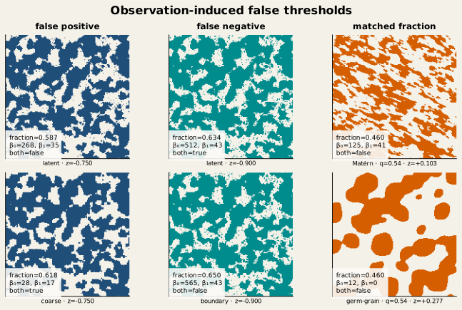
The gallery below uses deterministic explanatory selections rather than new performance estimates. On held-out Ising field 024, coarse observation at $z=-0.750$ changed latent non-spanning into observed both-direction spanning; boundary texture at $z=-0.900$ reversed a latent both-direction crossing into non-spanning. A separate Matérn/germ–grain pair had exactly the same recorded pond fraction, $0.4600$, but $(\beta_0,\beta_1)=(125,41)$ versus $(12,0)$.

A bounded MOSAiC case study

Synthetic fields provide controlled truth but cannot show every feature of real sea ice. The observational case uses the Fuchs and Birnbaum PANGAEA release for the MOSAiC Leg 4 floe. It contains 0.5 m orthomosaics and classified surface polygons for 30 June and 22 July 2020. The dataset’s change log matters: the corrected release replaced an erroneous July image, so the evidence record pins the downloaded file hashes rather than citing the DOI alone. Its CC BY 4.0 licence permits reuse with attribution, but the public site publishes only approved, non-geolocating derived diagrams and aggregate measurements.

The two dates are not treated as a dense time series. They are two observed morphologies within a changing physical system. The TIFFs are intersected in projected space, both polygon layers are rasterised to one shared $512^2$ grid, and analysis is conditioned further on the intersection of both classified-floe masks. Domain-aware Betti counts exclude unclassified pixels instead of treating them as ice; spanning uses the outer envelope of this irregular common domain. Differences can still reflect melt, drainage, deformation, and classification, so the study does not infer a seasonal percolation time.

The predeclared secondary check uses the Niehaus and Spreen Sentinel-2 melt-pond-fraction product only if date, projection, common-footprint, and scale checks pass. Those maps have 10 m cells containing fractional pond estimates, not 10 m binary photographs. Converting them to a binary network therefore introduces a new threshold and a mixed-pixel interpretation. A failed alignment or an absence of a compatible scene is reported as exclusion, not repaired by choosing a nearby date after seeing its pattern.

Niehaus and colleagues evaluated the Sentinel-2 retrieval using higher-resolution products and used it to document spatial and temporal variability. That work supports the use of the product as an observational scale comparison. It does not turn a fractional satellite pixel into latent pond topology. The case study therefore asks a modest question: which qualitative connectivity statements remain unchanged across defensible representations of these specific scenes?

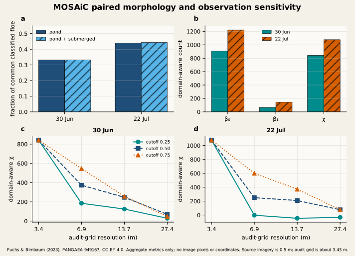
On the common $71{,}875$-cell classified-floe domain, the 30 June scene had pond fraction $0.3317$, $(\beta_0,\beta_1,\chi)=(907,65,842)$, and no horizontal or vertical crossing. The corrected 22 July scene had pond fraction $0.4399$, $(1223,146,1077)$, a horizontal crossing, and no vertical crossing; counting submerged ice with ponds changed its fraction only to $0.4429$. These summaries use the shared audit grid of about $3.427$ m per cell, not the native 0.5 m pixel label. They describe two representations, not a latent threshold or seasonal trend. Both matching-date Sentinel-2 requests returned HTTP 503, and the product metadata did not declare the floe-motion/co-registration transform needed for controlled pixelwise comparison. The satellite check was therefore excluded and no Sentinel-2 number is reported.

What this benchmark can and cannot teach us

The first lesson is methodological. Image resolution is not just a standard error around a fixed object. It changes the object on which a topological statistic is computed. A narrow bridge below the point-spread and sampling scale does not survive as a slightly uncertain bridge; it may become no bridge at all. Conversely, averaging can fill a narrow ice gap and create water connectivity. Observation therefore belongs inside the forward model.

Pond fraction, fractal scaling, Betti curves, spanning, and bottleneck width operationalise different events. Agreement is informative; disagreement reveals what the word “threshold” is actually naming.

The third lesson is about negative results. A method can rank first and still fail the predeclared all-strata robustness decision. That outcome would not show that the benchmark failed. It would show that the declared observation range is too demanding for threshold recovery from one binary image stack, or that additional temporal, spectral, or physical information is required.

The fourth lesson concerns scale. Persistent homology is multiscale, but a persistence diagram cannot restore information that the sensor never resolved. Stability to small perturbations of a filtering function is not invariance to destructive sampling. Topological tools help expose scale dependence; they do not abolish it.

Finally, compelling images invite causal stories about coalescence, drainage, or albedo. The synthetic experiment identifies only diagnostic response to a known operator; MOSAiC documents representation sensitivity. Explicit boundaries make both findings useful.

Limitations

The synthetic generators are varied but not exhaustive. They cannot represent every combination of snow topography, hydraulic routing, lateral melt, drainage, deformation, and refreezing. Robustness across them is not robustness across the Arctic.

The latent truth is operational: first finite-window spanning on a high-resolution raster under pond four-connectivity, expressed in latent pond fraction. Hydraulic, radiative, or ecological definitions could produce different thresholds. This truth audits image topology; it is not a universal physical order parameter.

Finite windows remain influential: a component can leave the crop, and an external path is invisible. Varying crop size cannot recover infinite-domain criticality from one floe. The triangular-lattice oracle validates code; it does not make correlated ponds independent site percolation.

Segmentation errors are stylised. The declared segmentation-bias stratum is exactly one observed-pixel outward grayscale dilation paired to the same mild random stream; it does not model inward displacement, spatially varying calibration, or a learned classifier. Real classifiers can have class-, texture-, and scene-dependent errors; clouds, shadows, submerged ice, reflection, and illumination may create structures outside the synthetic operator.

The public MOSAiC case has two dates, not a resolved transition trajectory. Alignment to a common footprint does not hold the physical floe fixed in every relevant respect. The Sentinel-2 product contains fractional estimates at a much coarser scale. Neither source supplies unobserved latent labels, so the observational analysis cannot validate the synthetic error magnitudes as empirical truth.

Persistent-homology and fractal estimates require analyst choices: filtration, boundary treatment, persistence pruning, the fixed $96^2$-maximum PH compute grid, scaling interval, minimum component size, and breakpoint rule. Freezing those choices protects held-out evaluation, but does not make them uniquely correct. The article reports sensitivity rather than hiding it.

Bootstrap intervals describe sampled latent-field variation under the declared design. They exclude generator structure, melt physics, and unmodelled observational systematic uncertainty. Claims remain restricted to the benchmark and bounded case.

A practical audit for future image studies

Before reporting a connectivity transition, specify phase classes, domain, pixel scale, adjacency, boundary condition, spanning direction, and whether the threshold is indexed by time, water level, area fraction, or channel radius. A final plot cannot recover these choices.

Place the observation pipeline between the physical hypothesis and statistic. Test plausible blur, resampling, segmentation-boundary displacement, boundary texture error, and crop on paired versions of the same field. If observation choices move the threshold more than the scientific comparison does, say so.

Use several summaries without voting after seeing the answer. Direct spanning, area, shape, and multiscale topology illuminate different failures. Predeclare the primary estimator and supporting diagnostics.

Count unresolved estimates. A missing breakpoint, exhausted computation, or scene without a defensible common footprint is data. Dropping such cases rewards a method for failing on difficult inputs.

Separate implementation verification from scientific validation. Exact masks and lattice checks can verify code, not establish the right physical description of drainage or albedo. A real-data illustration adds relevance, not latent truth.

Conclusion

A melt-pond threshold is never observed without an instrument, a pixel grid, a classifier, a window, and a definition of connection. The sharpness that makes topology attractive also makes it vulnerable: one erased or invented channel can reverse the conclusion while barely changing total area.

This study turns that vulnerability into an experiment. High-resolution synthetic fields provide a frozen latent target; paired observation operators separate morphology from measurement; six diagnostic families compete under the same held-out gate; exact fixtures and convergence tests audit the implementation; and a limited MOSAiC case shows how to carry the caution into real imagery.

The evidence does not identify a universally resolution-robust diagnostic. Raw spanning is the most accurate pooled estimator here, yet a single observed-pixel boundary displacement is enough to break its all-strata gate. The defensible conclusion is therefore not a preferred Arctic threshold, but a rule: report the observation operator, preserve tail failures, and abstain when connectivity does not survive it.

References

1. C. Polashenski, D. Perovich, and Z. Courville (2012). “The mechanisms of sea ice melt pond formation and evolution.” Journal of Geophysical Research: Oceans, 117, C01001. https://doi.org/10.1029/2011JC007231
2. C. Hohenegger, B. Alali, K. R. Steffen, D. K. Perovich, and K. M. Golden (2012). “Transition in the fractal geometry of Arctic melt ponds.” The Cryosphere, 6, 1157–1162. https://doi.org/10.5194/tc-6-1157-2012
3. P. Popović, B. B. Cael, M. Silber, and D. S. Abbot (2018). “Simple Rules Govern the Patterns of Arctic Sea Ice Melt Ponds.” Physical Review Letters, 120, 148701. https://doi.org/10.1103/PhysRevLett.120.148701
4. Y. Ma, I. Sudakov, C. Strong, and K. M. Golden (2019). “Ising model for melt ponds on Arctic sea ice.” New Journal of Physics, 21, 063029. https://doi.org/10.1088/1367-2630/ab26db
5. W. Offord, M. Coughlan, I. J. Hewitt, H. A. Harrington, and G. Grindstaff (2022). “Topological Data Analysis Detects Percolation Thresholds in Arctic Melt-Pond Evolution.” arXiv:2212.07961. https://arxiv.org/abs/2212.07961
6. V. Robins, M. Saadatfar, O. Delgado-Friedrichs, and A. P. Sheppard (2016). “Percolating length scales from topological persistence analysis of micro-CT images of porous materials.” Water Resources Research, 52, 315–329. https://doi.org/10.1002/2015WR017937
7. D. Cohen-Steiner, H. Edelsbrunner, and J. Harer (2005). “Stability of persistence diagrams.” Proceedings of the 21st Annual Symposium on Computational Geometry, 263–271. https://doi.org/10.1145/1064092.1064133
8. H. Edelsbrunner, D. Letscher, and A. Zomorodian (2002). “Topological persistence and simplification.” Discrete & Computational Geometry, 28, 511–533. https://doi.org/10.1007/s00454-002-2885-2
9. N. Fuchs and G. Birnbaum (2023). “Orthomosaics and surface type classifications of MOSAiC Leg 4 floe (2020-06-30, 2020-07-22).” PANGAEA dataset. https://doi.org/10.1594/PANGAEA.949167
10. H. Niehaus and G. Spreen (2022). “Melt pond fraction on Arctic sea-ice from Sentinel-2 satellite optical imagery (2017–2021).” PANGAEA dataset. https://doi.org/10.1594/PANGAEA.950885
11. H. Niehaus, G. Spreen, G. Birnbaum, L. Istomina, E. Jäkel, F. Linhardt, N. Neckel, N. Fuchs, M. Nicolaus, T. Sperzel, R. Tao, M. Webster, and N. Wright (2023). “Sea Ice Melt Pond Fraction Derived From Sentinel-2 Data: Along the MOSAiC Drift and Arctic-Wide.” Geophysical Research Letters, 50, e2022GL102102. https://doi.org/10.1029/2022GL102102
12. X. Miao, H. Xie, S. F. Ackley, D. K. Perovich, and C. Ke (2015). “Object-based detection of Arctic sea ice and melt ponds using high spatial resolution aerial photographs.” Cold Regions Science and Technology, 119, 211–222. https://doi.org/10.1016/j.coldregions.2015.06.014
13. C. Polashenski, K. M. Golden, D. K. Perovich, E. Skyllingstad, A. Arnsten, C. Stwertka, and N. Wright (2017). “Percolation blockage: A process that enables melt pond formation on first year Arctic sea ice.” Journal of Geophysical Research: Oceans, 122, 413–440. https://doi.org/10.1002/2016JC011994
14. M. Nicolaus, C. Katlein, J. Maslanik, and S. Hendricks (2012). “Changes in Arctic sea ice result in increasing light transmittance and absorption.” Geophysical Research Letters, 39, L24501. https://doi.org/10.1029/2012GL053738. The published correction revises absolute irradiance values while retaining the stated relative-flux conclusions; this article does not use the corrected values quantitatively.