Production Inside a Robust CSTR Safety Envelope

An exothermic continuous stirred-tank reactor is a compact lesson in nonlinear decision-making. Faster reaction raises conversion, but released heat accelerates the Arrhenius rate, which releases still more heat. Cooling opposes that loop. Under some parameters, several steady temperatures can satisfy the same operating conditions; under uncertainty, a nominally attractive point can sit close to an undesirable hot branch.

The study asks:

How much nominal production must be sacrificed to keep a declared thermal-risk proxy below a prescribed level when heat transfer and kinetics are uncertain?

This wording contains two safeguards. “Declared proxy” means the risk event is a mathematical criterion, not an accident probability. “Synthetic” means the distributions and parameters are stress-test devices, not a fitted plant uncertainty model.

Coupled material and energy balances

For concentration $C$ and reactor temperature $T$ , a first-order Arrhenius CSTR can be written

\frac{dC}{dt}=\frac{C_f-C}{\tau}-k_0e^{-E/(RT)}C,

\frac{dT}{dt}=\frac{T_f-T}{\tau} +\frac{-\Delta H}{\rho C_p}k_0e^{-E/(RT)}C -k_c(T-T_c).

Residence time $\tau$ and coolant temperature $T_c$ are decision variables. Conversion is $X=1-C/C_f$ , while a space-time-yield proxy is $X/\tau$ . The nominal optimizer seeks high yield using central kinetic and heat-transfer values.

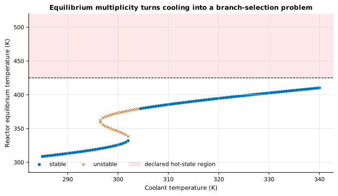
At steady state, the material balance gives concentration as a function of temperature. Substitution into the energy balance reduces equilibrium search to one scalar heat-balance residual. All roots over a declared temperature interval are found, then classified with the full two-state Jacobian. This matters because returning the first numerical root can hide multiplicity.

CSTR equilibrium branches and stability across operating conditions, with the nominal and robust choices marked. — **Figure 1.** The equilibrium landscape. A decision is interpreted relative to stable and unstable branches rather than from one solver return value.

Nominal optimum versus robust choice

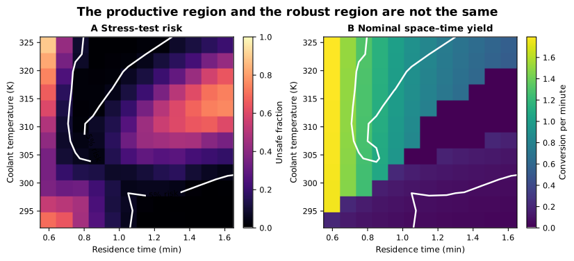
The nominal optimum uses residence time $0.55$ and coolant temperature $326$ . Its nominal conversion is $0.986$ , nominal yield $1.793$ , and equilibrium temperature about $434.25$ . Across the uncertainty ensemble, its declared risk is $0.8875$ .

The robust rule evaluates each candidate over uncertain heat-transfer and kinetic scenarios. A scenario is counted as risky if the declared hot-state or multiplicity criterion is triggered. The selected point uses residence time $0.75$ and coolant temperature approximately $319.82$ . Its nominal temperature falls to $411.67$ , conversion to $0.970$ , and yield to $1.293$ . Its ensemble risk is $0.01875$ .

That movement costs approximately $27.88\%$ of nominal yield. It is not a free robustness improvement; it is a quantified trade.

Decision map of residence time and coolant temperature showing yield and the robust feasible envelope. — **Figure 2.** Robust feasible envelope. The safest corner is not automatically selected: the decision maximizes the declared production objective subject to the risk constraint.

What probability means here

The value $0.01875$ is the fraction of 160 synthetic parameter scenarios that fail the declared equilibrium criterion. It is not a frequency estimate of fires, runaway, injuries, or loss. Such a claim would require plant-specific failure definitions, parameter posteriors, operating histories, protection layers, transient disturbances, and consequence models.

Scenario probability can still be useful. It forces an operating choice to survive a transparent collection of perturbations and provides a common scale for comparing decisions. But its interpretation is conditional on:

the uncertainty variables included;
their sampling distribution and dependence;
the hot-state threshold;
the equilibrium search range;
and the assumption that equilibrium behaviour is the relevant failure lens.

Changing any of those can move the envelope.

Equilibrium multiplicity is not the whole safety problem

A stable “cold” equilibrium and a stable “hot” equilibrium separated by an unstable branch produce classical ignition–extinction behaviour. Yet real reactor safety also depends on transients. Feed composition may jump; coolant can fail; controllers saturate; heat-transfer surfaces foul; mixing may be imperfect.

The current experiment uses equilibrium multiplicity and high stable temperature because they are auditable nonlinear markers. It does not simulate every disturbance trajectory. Consequently the robust choice should be read as robust against the declared parameter ensemble within an equilibrium model, not as a certified safe operating point.

Numerical verification

Root finding was repeated with 500, 1,200, 2,400 and 5,000 scan points. Each resolution found the same root for the verification configuration, with maximum residual about $5.68\times10^{-14}$ . Independent time integration approached the same equilibrium with temperature difference approximately $4.65\times10^{-10}$ .

Yield-risk frontier and numerical checks for the robust CSTR study. — **Figure 3.** Yield–risk trade-off beside root-resolution and time-integration checks. Numerical agreement supports the reported equilibrium calculations, not a plant-safety claim.

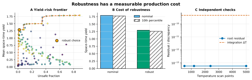
The scalar reduction and time integration fail differently. Root scanning can miss a narrow pair of equilibria if resolution is inadequate; time integration normally approaches only a stable equilibrium in the basin of its initial condition. Agreement therefore gives more information than repeating the same algorithm with a tighter tolerance.

The role of a held-out ensemble

Robust optimization can overfit scenarios just as a predictive model can overfit observations. If one repeatedly chooses a decision on the same random scenarios used to describe performance, the apparent risk can be optimistic.

The study separates the declared optimization ensemble from checks used to describe the selected point. A larger applied study should go further:

estimate uncertainty from an explicit data-generating process;
freeze the decision rule;
evaluate on independent posterior or stress scenarios;
report confidence intervals for violation probability;
include distribution shifts not represented during selection.

The current calculation demonstrates the workflow but does not claim full statistical calibration.

Why the nominal optimum is a useful failure case

It would be easy to dismiss the nominal optimum because its equilibrium temperature already exceeds the study threshold. That misses its methodological purpose. It is the result of optimizing exactly the production metric under nominal parameters. Its poor scenario performance shows what the objective omits.

A good baseline should be plausible and allowed to fail clearly. The robust method earns meaning only relative to that baseline:

nominal optimization achieves higher reported yield;
it is fragile under the declared uncertainties;
adding a risk constraint moves the decision;
the price of that movement is measured.

Without the yield sacrifice, “robust is safer” would be a one-sided claim. Without the nominal baseline, the robust point would have no decision context.

Sensitivity of the conclusion

The numerical values are sensitive to the synthetic parameter distributions and unsafe-temperature line. The structural conclusion is narrower and more stable: in a nonlinear exothermic CSTR, optimizing nominal yield can select a point with poor performance under uncertain heat removal and kinetics, and a scenario constraint exposes a measurable yield–risk frontier.

Important ablations for future work include:

heat-transfer uncertainty alone versus kinetic uncertainty alone;
independent versus correlated uncertainty;
equilibrium risk versus transient peak-temperature risk;
probability constraint versus worst-case or CVaR constraint;
fixed coolant temperature versus feedback control;
and alternative yield definitions including energy or material cost.

Each ablation changes a modeling choice rather than merely adding a larger optimizer.

Claim boundary

The experiment supports a reproducible mathematical statement about a synthetic reactor:

Under the declared balances, candidate grid, uncertainty ensemble, and thermal criterion, the robust point reduces scenario violation from $0.8875$ to $0.01875$ while surrendering $27.88\%$ of nominal yield.

It does not establish a safe operating envelope for a real plant. No operator should infer set-points from this article. Translating the workflow would require equipment-specific balances, calibrated kinetics and heat transfer, process hazard analysis, protection systems, transient validation, and formal engineering review.

References

R. Aris, Introduction to the Analysis of Chemical Reactors, Prentice-Hall, 1965.
W. H. Ray, Advanced Process Control, McGraw-Hill, 1981.
I. E. Grossmann and G. Guillén-Gosálbez, “Scope for the application of mathematical programming techniques in the synthesis and planning of sustainable processes,” Computers & Chemical Engineering, 2010. doi:10.1016/j.compchemeng.2009.11.012.
A. Ben-Tal, L. El Ghaoui, and A. Nemirovski, Robust Optimization, Princeton University Press, 2009. doi:10.1515/9781400831050.