When a Numerical Method Creates Negative Matter

Negative population, negative concentration, and negative compartment mass are often blamed on a model. Sometimes the differential equation is physically admissible and the impossibility is introduced by the time integrator.

This benchmark asks:

Under stiffness and coarse observation intervals, when do standard explicit schemes create impossible negative states, and what accuracy and cost are traded for a positivity- and mass-preserving update?

The experiment uses linear conservative transfer networks. This narrow setting is intentional: exact matrix-exponential solutions are available, positivity and conservation are mathematically transparent, and failure can be attributed to the numerical method rather than an ambiguous application model.

A conservative transfer network

Let $y_i(t)\ge0$ be material in compartment $i$. Transfers are encoded by a generator matrix $Q$:

Off-diagonal entries of $Q$ are non-negative, so one compartment cannot send a negative inflow to another. Column sums are zero, so

The exact solution $y(t)=e^{tQ}y(0)$ remains non-negative and conserves total mass. A numerical method should ideally preserve those structural facts.

Forward Euler gives

It is conservative because the column sums still cancel. But positivity requires every entry of $I+\Delta tQ$ to be non-negative, imposing a step-size restriction tied to the fastest outflow. In a stiff network, that restriction may be far smaller than the reporting interval.

Classical RK4 has much better local accuracy for smooth nonstiff problems, but it is not unconditionally positivity preserving. A high-order polynomial approximation to $e^{\Delta tQ}$ can contain negative entries or become explosively unstable outside its stability region.

The comparison method is a linearly implicit Patankar-type update:

For a conservative Metzler generator, the inverse has the required non-negative structure and preserves the mass sum. It resembles backward Euler, with first-order accuracy but strong feasibility properties.

The benchmark grid

The study varies rate scale, stiffness ratio, and step size across 429 cases. Every method starts from the same non-negative initial state and is evaluated against the matrix exponential. For each run it records:

• whether any state becomes negative;
• maximum total-mass error;
• relative trajectory error;
• computational work;
• and whether the calculation remains finite.

This design prevents a visually selected example from carrying the claim. The key result is a failure-rate surface.

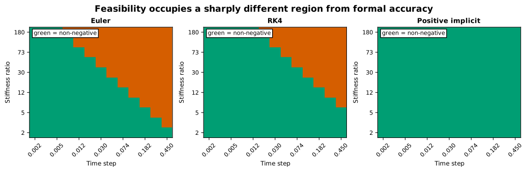
Across all 429 cases, Euler produces at least one negative entry in $38.46\%$ of runs and RK4 in $25.17\%$. The positive implicit method produces none.

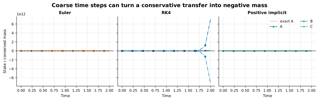
For unstable explicit runs, mass error can become enormous: maxima reach about $1.0\times10^{27}$ for Euler and $3.7\times10^{75}$ for RK4. Algebraically, explicit schemes preserve the column-sum invariant in exact arithmetic. Numerically, once an unstable trajectory grows to huge opposing values, floating-point cancellation and overflow destroy that property. The positive implicit method keeps maximum mass drift near $8.7\times10^{-14}$.

This distinction is important. “The method is conservative” as an algebraic formula is not the same as “the computed trajectory conserves mass in the tested regime.”

Positivity is not accuracy

The positive method avoids impossible states, but it is only first order. Large steps can smear fast transients. A solution that stays positive and conserves mass can still have substantial trajectory error.

The study therefore adds step doubling. One full step is compared with two half steps; their difference estimates local error and adapts $\Delta t$. Across tolerances from $2\times10^{-2}$ to $5\times10^{-4}$, accepted steps increase from 15 to 75 while relative error falls from approximately $0.0312$ to $0.00626$. All adaptive runs remain non-negative and keep mass error near machine precision.

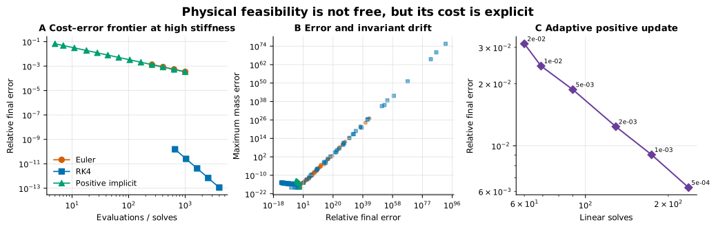
The trade-off is now explicit:

• Euler is cheap per step but can require a severe positivity/stability restriction.
• RK4 is accurate in its stable regime but uses four derivative evaluations and still lacks unconditional positivity.
• The implicit update requires a linear solve and is first order, yet preserves feasibility for the tested generator family.
• Step doubling improves error control at the price of multiple solves.

Why clipping is not the same solution

A common repair is to replace negative states by zero after each step. Clipping restores a visible inequality but generally changes total mass and hides the size of the numerical failure. Renormalising after clipping restores the sum but redistributes the error globally, creating a new undocumented method.

Structure-preserving integration differs because the update itself respects the invariant. That makes error interpretable: remaining discrepancy is mainly time-discretization error rather than a mixture of integration, clipping, and renormalisation.

Clipping can be defensible in an observation or projection model when explicitly formulated. It should not be silently used to make an unstable integrator look physical.

What stiffness is doing

Stiffness means the network contains widely separated time scales. Fast transfers can equilibrate long before slow circulation changes appreciably. Accuracy at the slow scale does not permit an explicit method to ignore the fast stability restriction.

In this benchmark, increasing the rate ratio shrinks the safe Euler step. RK4 has a larger stability region but not an unlimited one. The implicit update damps fast modes without requiring the step to resolve their stability scale, although resolving them may still be necessary if their transient shape is scientifically important.

This is why method choice must follow the question. If only long-time compartment totals matter, damping a fast transient may be acceptable. If the transient peak triggers a decision, first-order implicit smoothing may be unacceptable even though every state is positive.

Verification strategy

The matrix exponential provides an independent solution for the linear benchmark. Tests also verify:

• columns of $Q$ sum to zero;
• off-diagonal rates are non-negative;
• each method uses the same time grid in fixed-step comparisons;
• mass and minimum state are computed from unrounded trajectories;
• adaptive tolerance tightening produces decreasing reference error in the reported range.

The benchmark deliberately does not prove a theorem for nonlinear chemical kinetics. In nonlinear production–destruction systems, a Patankar method must weight transfers carefully, and order conditions become more involved.

Claim boundary

The supported statement is:

On the declared family of stiff linear conservative transfer networks, coarse explicit Euler and RK4 frequently produce negative or unstable trajectories, while the linearly implicit update preserves non-negativity and mass in all 429 tested cases; adaptive step doubling reduces its reference error at increasing solve cost.

This does not show that the implicit update dominates every high-order positivity-preserving, exponential, splitting, or nonlinear solver. It also does not imply that every negative model state is numerical—some governing equations themselves fail to preserve positivity.

A practical decision checklist

Before choosing an integrator for positive quantities:

1. Write the invariants. Which sums, bounds, or signs does the continuous system preserve?
2. Check whether the method preserves them conditionally or unconditionally.
3. Estimate the fastest time scale, not only the output interval.
4. Use an independent reference on a representative smaller problem.
5. Report minimum state and invariant drift beside ordinary error.
6. Do not repair silently. If projection or clipping is part of the algorithm, name and test it.
7. Match error to the decision. Long-time mass error and transient-peak error are different objectives.

References

1. E. Hairer, C. Lubich, and G. Wanner, Geometric Numerical Integration, 2nd ed., Springer, 2006. doi:10.1007/3-540-30666-8.
2. S. Kopecz and A. Meister, “On order conditions for modified Patankar–Runge–Kutta schemes,” Applied Numerical Mathematics, 2018. doi:10.1016/j.apnum.2018.01.004.
3. H. M. Munthe-Kaas, A. Zanna, and collaborators, structure-preserving methods discussed in the broader geometric integration literature.
4. R. J. LeVeque, Finite Difference Methods for Ordinary and Partial Differential Equations, SIAM, 2007. doi:10.1137/1.9780898717839.