Research Notes

When Sustainable Harvesting Becomes a Trap

A stochastic strong-Allee model shows why average sustainable yield can conceal a collapse threshold and why a feedback refuge changes the finite-horizon risk–yield frontier.

24 July 2026 · 20 min read

A harvesting rule can appear sustainable in an average year and still be dangerous.

The difficulty is not merely that environmental conditions fluctuate. If a population experiences a strong Allee effect—negative per-capita growth below a critical abundance—a temporary decline can cross a boundary after which recovery is no longer expected. A policy designed around mean carrying capacity may therefore fail through the interaction of seasonality, random shocks, and inflexible extraction.

This synthetic study compares a fixed quota, proportional harvesting, and a threshold-adaptive refuge rule. It asks a risk-aware question: which policy delivers useful harvest while keeping the estimated probability of finite-horizon collapse below an acceptable level?

It is not a stock assessment and is not calibrated to a named species. The model is deliberately compact so that the mechanism and the limitations remain visible.

A population with two density thresholds

Let (P_t) denote population abundance after harvesting at time (t). The update is

Pt+1=max{0,  Pt+rPt(1PtKt)(PtL1)Ht}.P_{t+1} = \max\left\{ 0,\; P_t+ rP_t\left(1-\frac{P_t}{K_t}\right) \left(\frac{P_t}{L}-1\right) -H_t \right\}.

The logistic factor (1-P_t/K_t) limits growth near carrying capacity. The Allee factor (P_t/L-1) is negative below the critical level (L). Thus the model has two qualitatively different low-population regimes: above (L), reduced abundance may recover; below (L), deterministic growth pushes downward.

Environmental capacity varies as

Kt=K0[1+Asin(2πtT)+σεt],εtN(0,1),K_t=K_0\left[ 1+A\sin\left(\frac{2\pi t}{T}\right)+\sigma\varepsilon_t \right], \qquad \varepsilon_t\sim N(0,1),

with a numerical lower bound to keep (K_t) positive. The sinusoid creates predictable seasons; the Gaussian term changes how severe each season becomes.

The default experiment uses

P0=70,r=0.2,K0=100,A=0.25,T=12,σ=0.06,L=20.P_0=70,\quad r=0.2,\quad K_0=100,\quad A=0.25,\quad T=12,\quad \sigma=0.06,\quad L=20.

Each policy-intensity setting is evaluated with 150 stochastic replicates over 200 time steps. Common random numbers are used so that policy comparisons share environmental sequences.

Three policies encode three responses

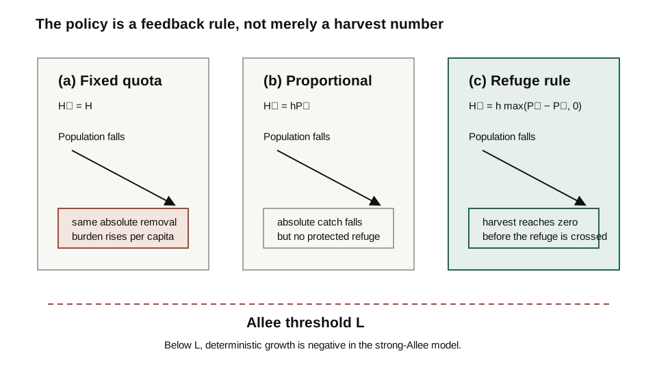
A fixed quota requests the same absolute amount:

Ht=H.H_t=H.

Its operational target is predictable, but the per-capita burden rises as the stock falls.

Proportional harvesting requests a fraction of current abundance:

Ht=hPt.H_t=hP_t.

Absolute extraction decreases automatically when the stock is small, although no abundance is explicitly protected.

The threshold-adaptive rule removes a fraction of the surplus above refuge (P_s):

Ht=hmax(PtPs,0),H_t=h\max(P_t-P_s,0),

with (P_s=60) in the default experiment. Harvest stops at or below the refuge.
Population trajectories under fixed-quota, proportional, and threshold-adaptive harvesting with the Allee and refuge thresholds marked.
Figure 1. Representative trajectories make the feedback difference visible. Once a fixed extraction helps push abundance below the strong-Allee threshold, the model's own dynamics reinforce the decline; the refuge rule stops extraction earlier.

This framing matters because a policy is not just a parameter. It is a mapping from observed state to action. The refuge rule can buffer the Allee threshold only if abundance is observed accurately and action is timely.

The risk cliff

Two outputs are recorded:

p^ext=runs reaching Pt<1simulation runs,\widehat p_{\mathrm{ext}} = \frac{\text{runs reaching }P_t<1} {\text{simulation runs}},

and mean realized harvest per time step, (\overline Y). These metrics must remain separate. A large requested catch can produce little realized long-run yield if the stock collapses early.

The fixed-quota grid shows an abrupt transition. Quota (H=7) produced one extinction in 150 runs; (H=8) produced 28; (H=9) produced 150. Mean yield rose from (6.98) to (7.23) between quotas 7 and 8, then fell to (1.89) at quota 9 because future catch disappeared.

The proportional rule also crossed a sharp boundary: (h=0.14) produced three extinctions in 150 runs and mean yield (8.86); (h=0.16) produced extinction in every run and mean yield only (1.63).

Across the tested threshold-adaptive grid, no run became extinct. At (h=0.8), mean yield reached (10.27). This is the strongest finite-horizon point in the supplied grid, not a proof that the policy is safe for all parameters or all time.
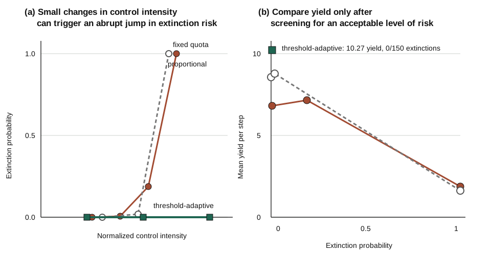
Estimated finite-horizon collapse probability against mean realized yield for fixed-quota, proportional, and threshold-adaptive harvesting.
Figure 2. Estimated risk and realized yield from 150 replicates per policy intensity. The threshold-adaptive rule occupies a favourable part of this tested grid, while small increases in the other controls cross a collapse boundary. Zero observed extinctions does not imply zero true risk.

The decision problem is better written as

maxθ E[Y(θ)]subject toPr(τextN)α,\max_\theta\ \mathbb E[Y(\theta)] \quad\text{subject to}\quad \Pr(\tau_{\mathrm{ext}}\le N)\le\alpha,

where (\theta) includes the policy family and its control, (N) is the planning horizon, and (\alpha) is a tolerated risk. Maximum average yield and robust sustainability are not the same objective.

Reading the experiment as a decision study

The simulation grid is easiest to interpret as a sequence of increasingly demanding questions.

First, does the unharvested model behave as intended? Above the Allee threshold, the population should be capable of returning toward the seasonally varying capacity; below it, per-capita growth should be negative. Second, does each controller implement the declared state-to-action rule? A fixed quota should not quietly become proportional when abundance is low, and the adaptive rule should not harvest below its refuge. Third, does a comparison use the same environmental evidence? Common random numbers make the policies experience the same 150 shock sequences at a given control level, reducing irrelevant Monte Carlo variation in pairwise comparisons.

Only after these mechanism checks does the risk-yield summary become meaningful. The supplied run contains 34 policy-intensity rows. Each row aggregates 150 trajectories, but it does not erase them: collapse counts, realized yield, and representative paths remain available as separate outputs. This matters because two policies with the same average harvest can reach it through very different histories.

PolicyControlCollapsesEstimated riskMean realized yield
Fixed quota7.001 / 1500.00676.984
Fixed quota8.0028 / 1500.18677.233
Fixed quota9.00150 / 1501.00001.894
Proportional0.143 / 1500.02008.864
Proportional0.16150 / 1501.00001.630
Threshold-adaptive0.800 / 1500.0000 observed10.274

The last row says that this finite experiment observed no collapse, not that the unknown collapse probability is exactly zero.

Zero events still have uncertainty

For a binomial event count (X\sim\mathrm{Binomial}(n,p)), the plug-in estimate (\hat p=X/n) is only one part of the result. When (X=0), a simple 95% upper rule of thumb is

pupper3n.p_{\mathrm{upper}}\approx \frac{3}{n}.

With (n=150), this is about (0.02). A Wilson interval gives a similar upper bound of roughly (0.025). Therefore “0 out of 150” is compatible with a small but non-zero finite-horizon risk. If the decision threshold were (\alpha=0.01), this experiment would be too small to certify it.

The change from 3/150 collapses at proportional control (0.14) to 150/150 at (0.16) is too large to be sampling noise alone, but the location of the transition is resolved only at the tested grid spacing. Controls at (0.145), (0.150), and (0.155) could reveal a narrow transition band or a mixture of delayed collapses.

Finite-horizon collapse probability across normalized harvesting intensity for fixed-quota, proportional, and threshold-adaptive policies.
Figure 3. Normalising control intensity makes the policy families easier to compare, but it does not make their actions equivalent. The sharp changes motivate local grid refinement and interval estimates for every risk point.

More replicates are most valuable near the decision boundary, not at settings that already collapse in every run. Sequential simulation could stop early when a control is clearly unsafe and redirect computation toward points whose confidence interval overlaps the tolerated risk.

Why feedback changes the frontier

The adaptive controller changes the timing of extraction. Its derivative with respect to abundance is

HtPt={0,PtPs,h,Pt>Ps.\frac{\partial H_t}{\partial P_t} = \begin{cases} 0, & P_t\le P_s,\\ h, & P_t>P_s. \end{cases}

Below the refuge, harvesting no longer adds a downward force. Above it, extraction grows with surplus. This creates a buffer between the operational stopping point (P_s=60) and the biological threshold (L=20). The buffer absorbs some seasonal and random losses before the system reaches negative natural growth.

Fixed quotas have the opposite local geometry. The requested removal is constant while its fraction of abundance, (H/P_t), increases during a decline. Proportional harvesting is safer than a comparable quota in that respect, but it continues to remove a fraction below any biologically meaningful refuge.

Comparative synthetic performance of fixed-quota, proportional, and threshold-adaptive harvesting policies.
Figure 4. Requested control and realized outcome are different. Aggressive rules can lose future yield after collapse, while a refuge can preserve both stock and subsequent extraction in this parameter setting.

The experiment supports a conditional mechanism: when a strong Allee threshold exists, a correctly observed refuge can prevent extraction from amplifying low-abundance dynamics. It does not show that the chosen refuge is optimal, that threshold policies dominate under every growth law, or that enforcement is costless.

From a perfect state variable to a usable policy

A real rule acts on an estimate rather than on (P_t). Suppose log-scale observation error and a one-step delay give

P^t=Ptexp(ηt),Ht=hmax(P^t1Ps,0).\widehat P_t=P_t\exp(\eta_t),\qquad H_t=h\max(\widehat P_{t-1}-P_s,0).

Now the safety margin must cover the distance between refuge and Allee threshold, possible upward observation error, and the decline that can occur during the delay. A high nominal refuge may still harvest at the wrong time if surveys are biased or infrequent.

This suggests three design variables: the biological refuge, the monitoring schedule and observation model, and the control intensity above the refuge. Optimising only the third is incomplete. A stronger formulation would draw ((r,L,\sigma)) from an uncertainty set, simulate delayed noisy observations, and minimise worst-case or upper-tail collapse risk subject to a yield requirement. A hidden-state version could use a particle filter and make harvest depend on a conservative posterior quantile rather than a point estimate.

What would count as stronger evidence?

The present results answer a mechanism question with a controlled synthetic experiment. Several additions would move it toward a management analysis:

  • estimate growth, threshold, and environmental terms for a named stock, with uncertainty;
  • repeat the comparison under alternative Allee formulations, age structure, and spatial refuges;
  • include survey noise, missing seasons, delays, and non-compliance;
  • tune controls on one ensemble and evaluate a frozen policy on independent shocks;
  • report how risk changes across multiple planning horizons;
  • include monitoring cost, yield variability, collapse loss, and recovery time without hiding their weights.

These additions may change the ranking. That is why the current result remains a verified synthetic study rather than a recommendation for a real fishery.

Why the refuge is not a free guarantee

The adaptive rule uses true (P_t) without delay. A real manager observes a noisy proxy, perhaps

P^t=Pteηt.\widehat P_t=P_t e^{\eta_t}.

Positive error can trigger harvesting when true abundance is already too low. Delayed surveys can have the same effect. A refuge policy is therefore information-intensive: its apparent robustness may depend on monitoring quality.

The experiment also treats environmental shocks as independent, contains no age or spatial structure, and uses one strong-Allee equation. It omits demographic stochasticity, economic price variation, implementation error, and parameter uncertainty. Most importantly, the 200-step risk estimate is not an infinite-horizon persistence theorem. A policy with no observed collapse in 150 finite trajectories can still have positive long-run extinction probability.

Verification and the next research question

The full configuration produced 34 risk–yield summary rows, representative trajectories, four figure families, and an animation. Six unit tests, output validation, and the SHA-256 manifest check passed. These checks support the code and the reported synthetic summaries.

A stronger study would treat abundance as a hidden state and compare policies under filtering uncertainty. It could introduce autocorrelated environments, delayed control, alternative Allee mechanisms, and robust optimization over uncertain (r), (L), and (\sigma). Policy ranking should then be evaluated out of sample over several horizons rather than on one fixed parameter grid.

Conclusion

Environmental variation does not merely add noise around a sustainable mean. Near an Allee threshold, it can expose a nonlinear boundary between recovery and collapse.

The central modeling lesson is to evaluate a feedback rule over distributions of trajectories, not only at an average equilibrium. A policy should be judged by the yield it produces at an explicitly tolerated level of risk—and by the information required to keep its safeguards functioning.

References

  1. Ricker, W. E. (1954). Stock and recruitment. Journal of the Fisheries Research Board of Canada, 11(5), 559–623. https://doi.org/10.1139/f54-039
  2. May, R. M. (1976). Simple mathematical models with very complicated dynamics. Nature, 261, 459–467. https://doi.org/10.1038/261459a0
  3. Stephens, P. A., Sutherland, W. J., & Freckleton, R. P. (1999). What is the Allee effect? Oikos, 87(1), 185–190. https://doi.org/10.2307/3547011
  4. Lande, R. (1993). Risks of population extinction from demographic and environmental stochasticity and random catastrophes. The American Naturalist, 142(6), 911–927. https://doi.org/10.1086/285580
  5. Reed, W. J. (1979). Optimal escapement levels in stochastic and deterministic harvesting models. Journal of Environmental Economics and Management, 6(4), 350–363. https://doi.org/10.1016/0095-0696(79)90014-7
  6. Hilker, F. M., & Liz, E. (2020). Threshold harvesting as a conservation or exploitation strategy in population management. Theoretical Ecology, 13, 519–536. https://doi.org/10.1007/s12080-020-00465-8