What Must a Traffic Model Remember?

Two pictures of a ring road can show identical gaps between cars and still have different futures. In one, the following cars are closing in; in the other, they are falling behind. A photograph of headways has omitted velocity. No amount of precision in measuring that photograph makes the missing variable disappear.

Past observations can partly repair this omission. A sequence of gaps reveals whether a wave is growing, moving, or decaying. But useful history might encode an omitted variable, compensate for projection onto a few coordinates, or average measurement noise. A fitted history model can also magnify tiny errors that were harmless in the original simulation.

Stability asks a different question from short-term forecast accuracy. A predictor can track a trajectory while placing a growth rate on the wrong side of zero; a correct sign need not mean accurate amplitudes. The study keeps both diagnostics.

The study below uses a synthetic optimal-velocity ring model to separate those questions. Its main experiment contains 297 parameter cells, 8,910 clean trajectories, and 23,463 fitted model settings. The central finding is conditional: history improves several forecasting and stability diagnostics for the chosen incomplete observations, especially under observation noise, but neither the improvement nor the name Mori–Zwanzig establishes that a fitted autoregression has recovered an exact physical memory kernel.

See the project overview for a shorter account.

Real first-mode Fourier headway and velocity amplitudes show two homogeneous trajectories separating despite their identical initial headway amplitude. — Figure 1. Two homogeneous trajectories at mean headway 15 m and rate ratio 0.90 share their initial headway mode but have opposite velocity modes. The panels show the real parts of the canonical, 1/N-normalized first Fourier coefficients, in metres and metres per second. Different futures demonstrate the missing velocity information; these are wave amplitudes, not individual vehicle measurements.

A ring road with an explicitly chosen observation

There are 24 cars, with fixed labels around a ring. The variable $h_i$ is the actual gap ahead of car $i$ , and $v_i$ is its velocity. The next label is interpreted cyclically. The optimal-velocity model, following the setting introduced by Bando and colleagues [13], is

\dot h_i=v_{i+1}-v_i,\qquad \dot v_i=\alpha_i[V(h_i)-v_i],\qquad V(h)=30\frac{\tanh((h-25)/12)+\tanh(25/12)}{1+\tanh(25/12)}.

Headway is measured in metres and velocity in metres per second. The positive rate $\alpha_i$ , in inverse seconds, controls how quickly a driver relaxes toward the preferred speed. This is a deliberately simple car-following law. There is no lane changing, reaction-time distribution, anticipation of several vehicles, or calibration to measured traffic in this study.

The sum of the headways is constant because all velocity differences cancel around the ring. That conservation law is useful, but it does not guarantee positive gaps. Nonlinear simulations terminate if a gap reaches zero; they do not wrap positions modulo the road length and reinterpret a collision as a new positive gap. Invalid initial conditions are recorded separately. A model of congestion should not quietly become a model that permits cars to pass through one another.

Uniform flow has every gap equal to $h_*$ and every speed equal to $V(h_*)$ , even when drivers have different relaxation rates. The experiment uses mean headways of 12.5, 15, and 17.5 metres. Write $c=V'(h_*)$ . Linearization then measures how small deviations from this uniform state evolve.

To compare gaps and speeds without mixing their units, headway perturbations are divided by 12 metres and velocity perturbations by 30 metres per second. A real, orthonormal Fourier transform separates spatial waves. Only the conserved mean-headway coordinate is removed; the mean-velocity coordinate remains. The resulting state has 47 real coordinates. With vehicle labels starting at zero, the first complex Fourier amplitudes in physical units are

H=\frac{1}{N}\sum_{j=0}^{N-1}(h_j-h_*)e^{-2\pi i j/N},\qquad W=\frac{1}{N}\sum_{j=0}^{N-1}(v_j-V(h_*))e^{-2\pi i j/N}.

The retained real coordinates are $\sqrt{2N}$ times the real and imaginary parts of $H/12$ and $W/30$ . This specifies both amplitude normalization and the negative-sine convention. In the scaled coordinates,

w=\begin{pmatrix}\delta h/12\\\delta v/30\end{pmatrix},\qquad A_w=\begin{pmatrix}0&(30/12)D\\(12/30)c\Lambda&-\Lambda\end{pmatrix},\qquad B=T A_wT^{\mathsf T},\qquad TT^{\mathsf T}=I_{47}.

Here $(Dv)_i=v_{i+1}-v_i$ , and $\Lambda$ is the diagonal matrix of relaxation rates. The transform has 47 rows and 48 columns. Its projection removes a structural conservation direction, not a troublesome eigenvalue chosen after seeing the answer.

The standard observation retains four real coordinates: the cosine and sine components of the first headway wave and the corresponding two velocity components. A richer observation adds the second spatial wave, giving eight coordinates. A separate headway-only control observes just two. These are different information sets, so their comparison must be labelled as such. A four-coordinate model is not an approximation to the entire road in every possible sense; it is a predictor for a specified observable.

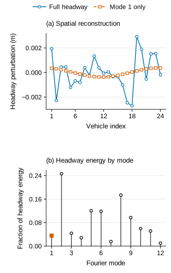
Full and first-mode reconstructed headway perturbations across 24 vehicles appear above the squared-coefficient energy fractions of the headway Fourier modes. — Figure 2. A held-out initial state at mean headway 15 m and rate ratio 0.90 is reconstructed across 24 vehicles. The first-mode curve keeps only the headway sine–cosine pair. The lower panel shows each mode's fraction of squared orthonormal headway coefficients, including the Nyquist mode. The mean headway perturbation is constrained to zero.

A closed pair and an incomplete photograph

Homogeneous drivers provide a negative control for claims about memory. If every relaxation rate equals $\alpha$ , Fourier modes decouple. For the first mode, let $H$ and $W$ denote the complex headway and velocity amplitudes in physical units, and put $a=e^{iq}-1$ , where $q=2\pi/24$ . Then

\dot H=aW,\qquad \dot W=\alpha(cH-W),\qquad \lambda^2+\alpha\lambda-\alpha ca=0.

Keeping both amplitudes gives an exactly closed linear system. Other spatial modes cannot add linear memory because they do not drive this pair. Four real coordinates determine its future, so a one-step matrix model fitted to noiseless, exact linear data should recover the closure to numerical precision.

This control prevents an easy but misleading story: a method that always benefits from additional lags has not thereby demonstrated unresolved traffic physics. In the homogeneous closed pair, any apparent advantage must be investigated through noise, finite precision, regularization, sampling, or the fitting procedure. Physical memory induced by discarded Fourier modes is absent there.

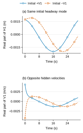
Now retain only headway. Solving the velocity equation and substituting it back gives

\dot H(t)=a e^{-\alpha t}W(0) +\alpha ca\int_0^t e^{-\alpha(t-s)}H(s)\,ds.

The first term remembers the hidden initial velocity. Two states can have the same $H(0)$ and different $W(0)$ , hence different initial headway derivatives. Dropping this term would replace exact trajectory reconstruction with a different prediction problem. An average over hidden initial states might be meaningful, but it would require a specified distribution and would not recover each individual trajectory.

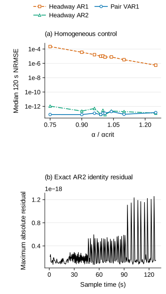
The integral has an exponential tail. It has no exact finite cutoff at which the past becomes irrelevant. Nevertheless, the sampled process has a short exact recurrence. If $E$ is the two-by-two complex state-transition matrix over one sampling interval, the Cayley–Hamilton identity yields

E=\exp\!\left[\Delta t\begin{pmatrix}0&a\\\alpha c&-\alpha\end{pmatrix}\right],\qquad H_{k+2}=\operatorname{tr}(E)H_{k+1}-\det(E)H_k,\qquad \det(E)=e^{-\alpha\Delta t}.

An infinite-tailed continuous memory can therefore have a finite recurrence representation. Here the recurrence is complex AR(2), equivalently a two-component real vector recurrence with two lags. It does not imply that a single real component must obey scalar real AR(2).

The experiment uses independent initial directions rather than putting every trajectory on one slow eigendirection. Even so, fast components can become very small by the forecast origin. This explains why headway-only AR(1) can perform well over the tested later interval without becoming an exact closure. Its homogeneous clean median error is about $1.06\times10^{-5}$ , whereas the two-lag headway control reaches about $2.20\times10^{-13}$ . Both scores concern two headway coordinates; neither belongs in a ranking of the four-coordinate predictors.

Homogeneous headway-only and closed-pair forecast errors are shown above the maximum residual of the exact complex two-lag recurrence. — Figure 3. Homogeneous controls: the upper panel shows median 120-second errors across three headways, after averaging each cell over 12 test trajectories. Headway AR1 and AR2 score two coordinates; pair VAR1 scores four, so this is not an equal-target ranking. Below, the exact complex AR2 recurrence residual is maximized over 30 trajectories at mean headway 15 m and rate ratio 0.90. It checks a floating-point identity, not a fitted residual.

Eliminating hidden coordinates does not eliminate their effects

Heterogeneity changes the projection problem. Each driver has rate $\alpha_i=\bar\alpha(1+\delta s_i)$ , with twelve signs $s_i=+1$ and twelve signs $s_i=-1$ . The values of $\delta$ are 0, 0.15, and 0.30. The mean rate is exactly $\bar\alpha$ , and its coefficient of variation is $\delta$ . Five fixed arrangements are examined for each nonzero level.

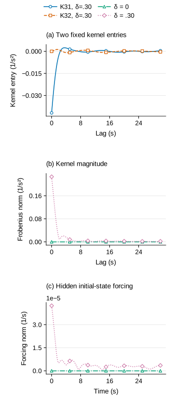
Different relaxation rates generally couple Fourier modes. The first headway–velocity wave is then driven by modes outside the four-coordinate observation. Partition the exact 47-dimensional linear system into retained coordinates $r$ and hidden coordinates $z$ . Variation of constants gives

\dot r(t)=B_{rr}r(t)+\int_0^tK(t-s)r(s)\,ds+f(t),\qquad K(t)=B_{rz}e^{B_{zz}t}B_{zr},\qquad f(t)=B_{rz}e^{B_{zz}t}z(0).

The instantaneous term describes what the retained state does directly. The convolution describes an excursion from retained to hidden coordinates and back. The forcing term carries the original hidden state. This is an exact coordinate-elimination identity, with every matrix specified by the traffic linearization and the chosen projection.

It is a concrete linear example of the separation that makes the Mori–Zwanzig viewpoint useful [1–4]. It is not a learned conditional-expectation projection, and no equilibrium fluctuation–dissipation formula is imported into the traffic model. The distribution used to generate initial conditions serves the numerical benchmark; it does not silently become a thermodynamic ensemble.

The hidden block also needs its own stability check. Stability of the full matrix does not, in general, imply stability of a block produced by an arbitrary projection. In the heterogeneous mechanism example, the maximum real part of the hidden-block eigenvalues is positive, about 0.00362 per second. There is therefore no basis for treating its kernel as a rapidly decaying exponential simply because that shape would be convenient for truncation.

Exact reconstruction is checked in two ways. An independent differential-equation calculation separates hidden motion driven by the retained state from motion arising from the hidden initial condition. A separate convolution calculation refines the quadrature step. Agreement with the full matrix-exponential trajectory, and convergence as quadrature is refined, test the identity more directly than an attractive overlay at one resolution.

Exact memory is not necessarily cheap: evaluating the hidden propagator still involves the hidden system. A finite-history regression can approximate its effects, but the fitted coefficients are not automatically the matrices in this exact kernel.

Three panels show two heterogeneous memory-kernel entries, complete kernel norms, and separate forcing norms from the hidden initial state. — Figure 4. Exact elimination at mean headway 15 m and rate ratio 0.90, using dimensionless-scaled coordinates. The panels show heterogeneous kernel entries K31 and K32, the full kernel Frobenius norm in inverse seconds squared, and hidden-initial-state forcing in inverse seconds. Homogeneous and 0.30-heterogeneity cases are compared. The homogeneous kernel vanishes analytically; numerical residues remain visible. A finite plotted interval does not imply finite memory support.

Driver order changes the projection, but not this full spectrum

The driver arrangements have a useful property that can be derived directly from this particular linearization. They need not share projected kernels, yet any permutation of the same relaxation-rate multiset has the same full-system eigenvalues.

For an eigenmode with exponent $\lambda$ , the velocity equation gives $h_i=(\lambda+\alpha_i)v_i/(c\alpha_i)$ . This divides by positive $c\alpha_i$ , not by $\lambda$ . Substitution into the headway equation gives a recurrence around the ring:

v_{i+1}=\left[1+\frac{\lambda(\lambda+\alpha_i)}{c\alpha_i}\right]v_i.

After one circuit, the velocity must return to its starting value. Multiplying the factors and clearing denominators produces the monic characteristic polynomial of the 48-dimensional physical Jacobian:

P(\lambda)=\prod_{i=1}^{N}(\lambda^2+\alpha_i\lambda+c\alpha_i) -\prod_{i=1}^{N}(c\alpha_i).

Multiplication does not depend on driver order. The polynomial is symmetric in the rates, so its roots depend on the multiset rather than the arrangement. Its zero root is simple because $P'(0)=N c^{N-1}\prod_i\alpha_i>0$ . That root corresponds to changing the uniform headway and speed together, outside the fixed-total-headway perturbation space. On the 47-dimensional physical manifold, the characteristic polynomial is $P(\lambda)/\lambda$ , understood as its polynomial extension at zero.

This is a direct derivation for the stated model, not a novelty claim or a universal fact about heterogeneous traffic. Changing the interactions, relaxation law, or driver-dependent parameters could invalidate the factorization.

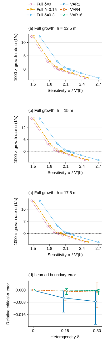
At fixed mean headway, heterogeneity level, and rate multiset, the five arrangements have the same true full-system boundary up to numerical error. Their spread cannot represent uncertainty in that boundary. Their eigenvector projections, observed kernels, and reduced-model errors can still differ.

Thus an observation can become a better or worse witness to the same instability without changing the instability itself. Full-system eigenvalues alone do not describe this visibility. A reduced observable with little component along a growing mode may reveal its growth weakly over a finite interval. Projection amplitudes are checked alongside the spectra for this reason.

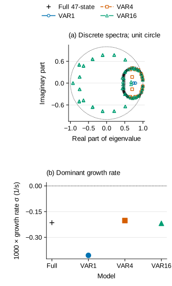
All full and fitted discrete eigenvalues are plotted against the unit circle above dominant growth rates for a fixed heterogeneous near-boundary case. — Figure 5. Full and learned spectra for mean headway 15 m, heterogeneity 0.30, arrangement 0, and rate ratio 1.01. Every eigenvalue of the full 47-state sampled map and VAR1, VAR4, and VAR16 appears against the unit circle. Sampling is 0.5 seconds; the lower panel compares dominant growth rates per second. Additional companion poles are not automatically physical traffic modes, and none is stabilized by clipping.

When does a traffic wave grow?

For the continuous linear system, stability is assessed by the largest real part of an eigenvalue. For a fitted discrete predictor, the corresponding diagnostic comes from the spectral radius of its augmented companion matrix. In the homogeneous ring, the first spatial mode supplies an analytical boundary:

s(B)=\max_{\lambda\in\sigma(B)}\operatorname{Re}\lambda,\qquad \widehat s=\frac{\log\rho(C)}{\Delta t},\qquad \alpha_c=c\left[1+\cos\!\left(\frac{2\pi}{N}\right)\right].

Here $C$ is the companion matrix, not a continuous generator obtained by choosing a matrix-logarithm branch. The sign of the growth diagnostic distinguishes decay from growth. It does not identify every feature of a wave, and the homogeneous boundary is a linear instability of uniform flow, not a universal threshold for finite-amplitude jams or hysteresis.

For heterogeneous systems, the full spectral abscissa is evaluated at 201 logarithmically spaced values of $\bar\alpha/c$ between 0.1 and 10. Every observed sign-changing interval is refined by a root solver. A finite scan is not a proof that there are no tangent roots or roots outside the interval. Cases without a detected crossing, or with several crossings, must remain distinguishable from a single verified crossing.

The main benchmark samples nine ratios to each detected critical mean rate: 0.75, 0.90, 0.96, 0.99, 1, 1.01, 1.04, 1.10, and 1.25. A tolerance of $10^{-6}$ per second defines marginal full-system growth. Exact-boundary cells are excluded from binary stable–unstable error counts, rather than assigning an arbitrary sign to numerical roundoff.

Clean comparisons have 240 non-marginal heterogeneous and 24 homogeneous cells; five noise realizations raise these denominators to 1,200 and 120. A classification mismatch includes a fitted marginal label for a non-marginal full system, not only opposite growth signs.

Learned boundary locations require another distinction. They are estimated by linear interpolation between the nine sampled rate ratios. These are grid-based estimates, whereas the reference boundaries are refined from the full-system spectral calculation. Their disagreement combines fitted dynamics and the finite parameter grid; the two root-finding procedures should not be presented as equally exact.

Three sampled full-system growth curves precede learned boundary errors with descriptive mean and min–max summaries across fixed settings. — Figure 6. The upper panels connect nine stored full-system growth samples for each heterogeneity level, using arrangement 0 at three mean headways. The bottom panel compares interpolated single-crossing estimates with refined full-system boundaries. Markers and whiskers are descriptive means and minima–maxima across three homogeneous systems or 15 systems per nonzero heterogeneity level, not confidence intervals. Only single crossings enter these averages. Permutations of a fixed rate multiset have identical true boundaries; any fitted-boundary spread concerns the reduced model.

What the forecast comparison actually measures

Every parameter cell has 12 training, six validation, and 12 test initial conditions. Each is an independent Gaussian direction in the 47-dimensional Fourier space, rescaled to a small physical nondimensional root-mean-square amplitude of $10^{-4}$ . Splitting occurs by complete trajectory before constructing lagged training rows. Adjacent times from one trajectory are not independent test examples.

Trajectories cover 128 seconds at half-second intervals. Forecasts begin at eight seconds and use only causal observations, with errors evaluated over 10-, 30-, and 120-second windows. Models are refitted for each parameter setting and arrangement; this tests local reduction, not transfer across traffic conditions.

A four-coordinate vector autoregression uses one, two, four, eight, or sixteen lags. The richer eight-coordinate model uses one lag. The headway-only controls and a one-lag total-least-squares diagnostic answer additional, explicitly separated questions. In general, the fitted recurrence is

\widehat r_{k+1}=\sum_{j=0}^{m-1}A_j\widehat r_{k-j}.

No intercept is fitted because the variables are perturbations about the known equilibrium. Each channel is scaled using training data alone. Ridge strengths range from zero through $10^{-10},10^{-8},10^{-6},10^{-4},10^{-2}$ , with a relative singular-value cutoff of $10^{-10}$ . The normalization of the fitting objective is fixed:

\min_{\Theta}\ \frac{1}{n}\lVert Y-X\Theta\rVert_F^2+\eta\lVert\Theta\rVert_F^2.

The factor $1/n$ matters: otherwise a change in the number of training rows would silently change the meaning of a ridge parameter. All methods share target times beginning at the maximum lag of sixteen. A shorter model does not receive additional early targets unavailable to the longer one.

Selection uses the mean of the 10- and 30-second validation-window normalized errors. Clean validation trajectories are available because this is a synthetic experiment. That advantage is disclosed rather than passed off as a deployment procedure for noisy roads with unknown truth. Test trajectories do not select regularization, lag order, or stability labels.

The test normalized root-mean-square error uses clean training-channel scales and is first computed per test trajectory. Summaries then aggregate the resulting errors across the fixed settings. The eight-coordinate model is scored on the same first four coordinates as the standard models, so adding four targets cannot improve its score by changing the question. Its additional input information remains an advantage and is not disguised as equal observational cost.

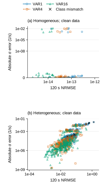
In the clean heterogeneous cells, one-lag VAR has median 120-second error 0.04043 and 12 classification mismatches out of 240 non-marginal cells. Two lags reduce the median to 0.02837 with no mismatches. Four lags reach 0.02119 but have two mismatches: one opposite sign and one fitted marginal label. Eight lags reach 0.01563 with none, while sixteen lags give 0.01664 with none.

Sixteen lags are not the best clean median, and improving median error from two to four lags does not improve the classification count. The two metrics examine different properties of the fitted dynamics. The richer one-lag observation has median error 0.02687 and three classification mismatches, illustrating another route to improvement: measure more of the state instead of extending the history of a fixed observation.

The homogeneous four-coordinate one-lag control reaches a median error near $8.49\times10^{-14}$ , as expected for an exactly closed, noiseless linear pair. This agreement supports the implementation and the analytical null case. It is not evidence that machine precision will be achievable with physical sensors.

Separate homogeneous and heterogeneous scatter plots compare clean forecast error with spectral-growth error and mark classification mismatches. — Figure 7. Clean 120-second forecast error versus absolute dominant spectral-growth error, separated into homogeneous and heterogeneous panels. Each point averages forecast error over 12 test trajectories for VAR1, VAR4, or VAR16. Black crosses mark classification mismatches outside the marginal tolerance of one millionth per second. Horizontal axes are logarithmic; symmetric-log vertical axes retain zero spectral error. A small observed-state error is not a full-system stability certificate.

Noise can make useful history look like physical memory

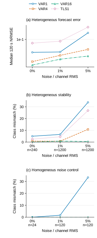
Observation noise is added at 1% and 5% of each clean training channel’s root-mean-square scale. Each nonzero level has five independent realizations. The noise streams are separate from the initial-condition draws, and all competing models share the same noisy observations within a realization. Both fitting data and the causal forecast warmup are noisy; the future reference remains the saved clean trajectory.

This tests measurement error, not random forcing in the car-following equations. Smoothing with observations after the forecast origin is forbidden: that would let the predictor use the future.

At 5% noise, the heterogeneous one-lag model gives 406 classification mismatches out of 1,200 non-marginal fitted settings and median error 0.15725. Sixteen lags give six classification mismatches and median error 0.03115. Eight lags lie between them, with 37 classification mismatches and median error 0.03878. This is strong evidence of a benefit within the tested design, not a guarantee about an untested noise distribution or a longer forecast horizon.

The homogeneous control is particularly informative here. It has no omitted-mode memory for the complete first-mode pair, yet longer histories also improve its noisy predictions. The sixteen-lag homogeneous median at 5% noise is 0.01084, compared with 0.14401 for one lag. A gain from history therefore cannot, by itself, diagnose a nonzero physical projection kernel.

Total least squares addresses another aspect of the problem. Ordinary regression treats predictors differently from responses, even though measurement noise contaminates both. The joint snapshot treatment motivating total DMD can reduce bias under appropriate assumptions [8]. Here a one-lag TLS fit is included as a noise-sensitivity diagnostic, with singular response blocks treated as failures rather than inverted regardless of conditioning.

It does not reliably rescue this benchmark. Across the full set of fitted settings, 88 nonfinite outcomes occur, all in TLS comparisons: 53 in heterogeneous 5% noise, 17 in homogeneous 1% noise, and 18 in homogeneous 5% noise. Large but finite errors also remain possible. The finite-only medians must therefore be read with the nonfinite counts, not used to make the failed runs disappear.

Lagged snapshots overlap, trajectories are transient, and signal strengths can differ greatly across directions. These conditions are not equivalent to independent, identically informative noisy samples. TLS is neither a universal denoiser nor a certificate that the recovered operator is physical. No fitted eigenvalues are clipped to make a model stable, and stability labels do not participate in hyperparameter selection.

Three noise panels show heterogeneous forecast error, heterogeneous misclassification percentages, and homogeneous misclassification percentages with their denominators. — Figure 8. Observation-noise stress without pole stabilization. Panels show heterogeneous median 120-second error, heterogeneous misclassification percentages, and homogeneous misclassification percentages for VAR1 and VAR16. Clean versus noisy sign denominators are 240 versus 1,200 for heterogeneous systems and 24 versus 120 for homogeneous systems; each nonzero noise level has five realizations. Errors average 12 test trajectories before aggregation. TLS uses the same observations and clean synthetic validation targets; finite medians must be read alongside the reported nonfinite outcomes.

Nonlinear stress tests expose a numerical limit too

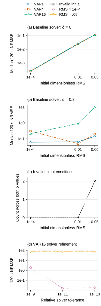
Linearization describes small perturbations near uniform flow. The nonlinear supplement reuses selected noise-free linear models without refitting. It fixes mean headway at 15 metres, uses homogeneous drivers or one 0.30-heterogeneity arrangement, and tests rate ratios 0.90, 0.99, 1.01, and 1.10. Twelve test directions are scaled to amplitudes $10^{-4}$ , 0.01, and 0.05.

There are 288 attempted trajectories. Two initial states fail the admissibility check because they contain negative velocities. The remaining 286 are valid integrations, with no zero-headway collision events in this set. Those counts describe this finite experiment, not a proof that the optimal-velocity model prevents collisions.

The nonlinear reference uses an adaptive high-order solver. Long-history prediction shows why deterioration against this reference cannot automatically be attributed to traffic nonlinearity: tiny errors in the observed warmup can be amplified even when the state trajectories look converged.

Consider one heterogeneous unstable case at rate ratio 0.90 and amplitude $10^{-4}$ . For the same sixteen-lag model and initial direction, the 120-second normalized error is 1.8371 with relative and absolute solver tolerances $10^{-9}$ and $10^{-11}$ . Tightening them to $10^{-11}$ and $10^{-13}$ changes the error to 0.01591. A still tighter calculation, at $10^{-13}$ and $10^{-15}$ , gives 0.01811. The exact linear comparison for this case is 0.02861.

The first value cannot support a clean claim that tiny physical nonlinearities destroyed the predictor. The forecast is sensitive to the numerical history supplied at its origin. Small state-space solver differences can have large effects after the recurrence repeatedly feeds its own predictions back into the delay state. Accuracy of the reference trajectory and robustness of a learned forecast are separate numerical questions.

At amplitude 0.05, the same representative case gives errors 72.8425, 72.8447, and 72.8448 across the three solver settings. Its severe degradation persists under refinement. That is evidence for a robust finite-amplitude limitation of this fitted predictor in this case, not evidence that every nonlinear failure in the entire sweep has the same cause.

This post-result tolerance study covers 24 representative case–amplitude combinations. It leaves the original 288 attempts intact and does not retune models. Its purpose is to identify a numerical confound before interpreting forecast degradation as physical mechanism.

This distinction affects how the figures should be read. A poor nonlinear score is an observation to explain, not a diagnosis on its own. To attribute it to nonlinear dynamics, one needs both a sufficiently converged reference and a predictor whose response to the remaining history error is understood.

Nonlinear forecast errors, invalid initial conditions, and a solver-tolerance comparison distinguish finite-amplitude degradation from numerical-history amplification. — Figure 9. Linear-trained models forecast nonlinear trajectories at initial RMS amplitudes 0.0001, 0.01, and 0.05 without refitting. Baseline medians pool 12 directions at four rate ratios, at mean headway 15 m, separately for homogeneous and 0.30-heterogeneous drivers. Only available finite 120-second errors enter medians. Panel (c) counts the two invalid initial states with negative velocities among 288 attempts; all 286 valid runs reach the full horizon without collisions. The final panel checks the same representative VAR16 case under tighter solver tolerances: tiny-amplitude error is numerically sensitive, while large-amplitude degradation persists. Shorter horizons never replace missing long-horizon scores.

History is measured in seconds, and it has a cost

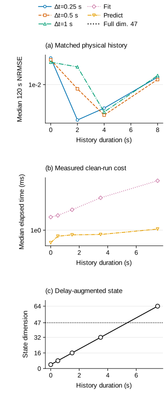
A lag count is not a physical memory duration. With half-second sampling, sixteen observations span 7.5 seconds because the current observation is included. Calling this an eight-second memory would conflate the available warmup interval with the model’s actual oldest lag.

For an unrestricted vector autoregression with observed dimension $d$ and $m$ lags,

T_{\mathrm{history}}=(m-1)\Delta t,\qquad p=d^2m,\qquad d_{\mathrm{aug}}=dm.

The standard one-lag model has 16 coefficients and a four-dimensional state. Sixteen lags raise these to 256 coefficients and a 64-dimensional augmented state. The eight-coordinate one-lag model has 64 coefficients and eight state coordinates, whereas four lags of the standard observation also have 64 coefficients but a sixteen-dimensional augmented state.

That equal coefficient count does not make the two models equivalent. One sees an additional spatial wave; the other sees a longer temporal record. Their regression conditioning and recurrence spectra can differ. Parameter counts, state dimensions, measured fitting time, and measured rollout time answer complementary cost questions rather than collapsing into one complexity score.

A supplementary sampling comparison uses intervals of 0.25, 0.5, and 1 second, while holding physical history at 0, 2, 4, or 8 seconds. Initial directions and forecast origin are matched, and target rows are common within each sampling case. An eight-second history therefore uses 33, 17, or nine observations depending on sampling, not the same lag count at every resolution.

This guards against calling finer sampling a longer physical memory. Sampling also changes parameter count and the closeness of adjacent observations. Any proposed optimal lag count therefore needs its sampling interval, observation definition, regularization, and forecast task.

The exact headway recurrence supplies an even sharper warning. Two complex lags can encode an exponential memory of infinite duration. Conversely, a long fitted delay vector can use its extra flexibility to fit noise-sensitive directions rather than the mechanism of interest. Neither “short” nor “long” is a property of traffic alone; it belongs to the representation and the task.

Three panels compare fixed physical histories at three sampling intervals, measured fitting and prediction times, and companion state dimensions. — Figure 10. Physical histories of 0, 2, 4, and 8 seconds are compared at sampling intervals 0.25, 0.5, and 1 second; points are medians over four fixed homogeneous/heterogeneous, stable/unstable cases. The middle panel reports measured fitting and 12-trajectory prediction times across clean main-run cells, not hardware-independent complexity. The bottom panel gives actual companion dimensions: main-run VAR16 uses 7.5 seconds and 64 state coordinates, exceeding the full model's 47.

What belongs to prior work, and what this experiment adds

Mori’s projection formulation [1] and Zwanzig’s memory viewpoint [2] provide the historical setting. The later correction by Zwanzig, Nordholm, and Mitchell [3] concerns neglected fluctuations in a nonlinear transport derivation; it is not a rejection of every projection identity. The traffic elimination above is checked directly rather than justified by invoking a famous name.

Chorin, Hald, and Kupferman [4] explain why exact memory need not be inexpensive and why short-memory approximations need conditions. The data-driven work of Yen Ting Lin and collaborators [5, 6] specifies projections, residual recursions, and generalized fluctuation relations, rather than merely fitting a delay equation.

That distinction limits the language used here. The present VAR coefficients are fitted jointly by delay regression. They are finite-history predictive proxies, not estimates certified to equal the exact coordinate-elimination kernel. The recursive operator-learning construction in [6] is a close methodological precedent, not a procedure reproduced merely by fitting several lags.

Kevin K. Lin and Fei Lu [7] connect history-based Wiener projections with reduced models and rational approximations. Moving the past into an enlarged state can remove an explicit memory integral without removing history dependence. Residual orthogonality also does not establish independent white noise. Those distinctions are useful when a compact recurrence is interpreted as physical evidence.

Memory-based reduction has also reached graph dynamics [9] and Lagrangian turbulence [10]. Those results remain application-specific: graph scaling arguments provide no universal cutoff for this car-following kernel, and turbulence forecasts do not validate traffic stability signs.

Traffic itself is not an untouched application. Tong and Ai’s 2026 traffic-prediction paper [11] explicitly describes an MZ-inspired operator architecture. The accessible publisher preview establishes that connection, although it does not permit a detailed audit of every projection claim. Chen and colleagues [12] study non-Markovian routing dynamics in which traversal duration depends on link-entry conditions. Remembering residual travel time is a different hidden-state problem from eliminating velocity or Fourier modes in a car-following model.

The contribution here is consequently an application-specific set of analytical controls and numerical comparisons. It shows where a closed state provides a null case, how a hidden variable creates exact memory and initial-state forcing, and why heterogeneity changes projected closure even when permutations preserve the full spectrum. The benchmark then measures the consequences for prediction, spectral signs, noise sensitivity, nonlinear stress, and numerical robustness.

All trajectories are synthetic, the parameter grid is finite, the initial ensemble is chosen, and models are refitted locally. Quantiles across fixed settings are not confidence intervals for real drivers; times within a trajectory are not independent replications. Zero sign errors in a subset do not establish a stability guarantee. No road-control intervention is evaluated.

Conclusion

The practical lesson is to ask what information the model has before asking how much memory it needs. For the homogeneous first-mode headway–velocity pair, exact linear closure already exists. For headway alone, history supplies omitted velocity information. For a heterogeneous projection, hidden modes contribute an exact memory term, but a useful finite-history fit remains an approximation. Under noise and finite precision, history can help the prediction and also create new sensitivities. Those distinctions are what make a memory model interpretable, rather than merely longer.

References

Mori, H. (1965). Transport, Collective Motion, and Brownian Motion. Progress of Theoretical Physics, 33(3), 423–455.
Zwanzig, R. (1961). Memory Effects in Irreversible Thermodynamics. Physical Review, 124(4), 983–992.
Zwanzig, R., Nordholm, K. S. J., and Mitchell, W. C. (1972). Memory Effects in Irreversible Thermodynamics: Corrected Derivation of Transport Equations. Physical Review A, 5, 2680.
Chorin, A. J., Hald, O. H., and Kupferman, R. (2002). Optimal prediction with memory. Physica D, 166(3–4), 239–257.
Lin, Y. T., Tian, Y., Livescu, D., and Anghel, M. (2021). Data-Driven Learning for the Mori–Zwanzig Formalism: A Generalization of the Koopman Learning Framework. SIAM Journal on Applied Dynamical Systems, 20(4), 2558–2601.
Lin, Y. T., Tian, Y., Perez, D., and Livescu, D. (2023). Regression-Based Projection for Learning Mori–Zwanzig Operators. SIAM Journal on Applied Dynamical Systems, 22(4), 2890–2926.
Lin, K. K., and Lu, F. (2021). Data-driven model reduction, Wiener projections, and the Koopman-Mori-Zwanzig formalism. Journal of Computational Physics, 424, 109864.
Hemati, M. S., Rowley, C. W., Deem, E. A., and Cattafesta, L. N. (2017). De-biasing the dynamic mode decomposition for applied Koopman spectral analysis of noisy datasets. Theoretical and Computational Fluid Dynamics, 31(4), 349–368.
Yu, Y., Harlim, J., Huang, D., and Li, Y. (2025). Learning coarse-grained dynamics on graph. Physica D, 481, 134801.
de Wit, X. M., Gabbana, A., Woodward, M., Lin, Y. T., Toschi, F., and Livescu, D. (2026). Data-driven Mori–Zwanzig modeling of Lagrangian particle dynamics in turbulent flows. Proceedings of the National Academy of Sciences, 123(13), e2525390123.
Tong, H., and Ai, Q. (2026). A deep spatio-temporal Graph Attention Network to learn nonlinear operators for traffic prediction. Physica A, 697, 131741.
Chen, J., Hu, M., Li, M., Chen, F., and Cao, J. (2026). Routing-induced phase transitions in traffic efficiency of non-Markovian dynamics. Physical Review Research, 8, L012021.
Bando, M., Hasebe, K., Nakayama, A., Shibata, A., and Sugiyama, Y. (1995). Dynamical model of traffic congestion and numerical simulation. Physical Review E, 51(2), 1035–1042.