Did the Hotspot Move, or Did It Grow?

Imagine two aerial maps of an algal bloom. In the first, the strongest patch lies towards the left of a narrow channel. In the second, the right-hand patch has become stronger while the left-hand patch has faded. Did material travel between them? Did organisms grow where conditions improved and disappear elsewhere? Or did both things happen?

A difference map identifies where the image changed. A transport map goes further: it draws a correspondence between the two distributions. That extra structure is attractive because it resembles an explanation. Arrows suggest motion; a source term suggests growth. Once the picture looks physically plausible, it is easy to forget that the intermediate history was never observed.

This article studies that distinction in a deliberately small synthetic world. There are no satellite observations, biological measurements or fitted ecological parameters. The maps are smooth positive fields on a periodic one-dimensional domain. We choose their generating histories, keep those histories hidden from the estimator, and ask what an established unbalanced optimal transport method actually tells us.

The answer is useful but narrower than a reconstructed history. The method finds a compromise under a specified cost model. Sometimes its allocation between transport and marginal change agrees with the action budget of our chosen history. Sometimes it does not. Most importantly, two very different histories can have exactly the same starting and finishing maps. In that situation, solving the optimization problem more accurately cannot tell us which history occurred.

The project overview gives a shorter account. Here we develop the model, inspect eight figures, and work out which additional observations would change the question.

What the comparison found

The experiment contains 4,320 entropic UOT fits, covering 180 labelled endpoint cases, three geometries and a fixed set of cost parameters. All of those fits meet the declared numerical convergence criteria. This is a deterministic design grid, not 4,320 independent observations of nature.

Convergence does not establish a physical interpretation. With the stated label convention, the static cost-share label agrees with the generating action label in 62.50% of nontrivial pure-translation configurations and 29.17% of nontrivial uniform-growth configurations. Those percentages describe this particular grid and this particular diagnostic; they are not deployment accuracies for an environmental monitoring system.

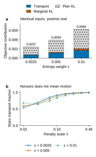
An even simpler warning needs no classification threshold. When the initial and final maps are identical, the chosen generating history has no motion and no growth. Yet the regularized coupling still carries positive transport cost. In one illustrated setting its transport share is 99.29%. The denominator contains small algorithmic costs, not evidence of substantial physical activity.

The strongest result is an ambiguity, rather than a ranking. We construct endpoint pairs compatible with both a moving history and a stationary growth-and-decay history. The two histories remain indistinguishable to every estimator that receives only those endpoints and the same auxiliary information. UOT is not uniquely responsible for this limitation; it makes the limitation particularly visible because its output is so easy to read as a physical explanation.

Four ways to change a map

Our spatial coordinate runs from zero to one and wraps around. Positions near zero and one are neighbours. This circle avoids boundary inflow and outflow, which would otherwise add another mechanism for changing total mass. It is a modelling convenience, not a claim that a real channel forms a closed ring.

Each initial density consists of two smooth periodic peaks with relative weights 1 and 0.65. We use three peak separations, with centres at (0.28, 0.46), (0.28, 0.58) and (0.28, 0.72). The width parameter is 0.045. Smooth periodic peaks avoid introducing an artificial derivative discontinuity where the coordinate wraps around.

The main grid has 256 cells. Each cell stores mass, so a density value is multiplied by the cell width before entering the transport problem. Omitting that factor would change the meaning of the objective when the grid is refined. Requested translations are rounded to the nearest cell and their actual displacement is retained. For example, a requested shift of 0.10 becomes 26/256, or 0.1015625.

The first family translates the whole field and preserves total mass. The second multiplies the field by a constant without moving anything. The third translates while applying a smoothly varying local growth factor. The fourth swaps the weights of the two peaks, optionally adding translation and a change in total mass. That last family will support two different histories.

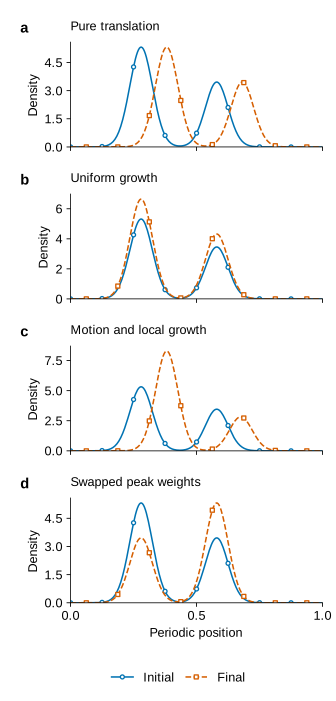
Four vertically arranged pairs of initial and final periodic density curves show translation, uniform growth, mixed change and swapped peak weights. — Figure 1. Four controlled changes on the 256-cell circle, using initial peak centres 0.28 and 0.58. Blue circles and solid lines denote initial density; orange squares and dashed lines denote final density. Translation uses an actual shift of 0.1015625 and unchanged total mass. Uniform growth has mass ratio 1.25 and zero shift; mixed change combines the same shift with spatially varying growth and mass ratio 1.25. The swapped-weight example has unchanged total mass and no added global shift. Curves are saved experimental endpoints, not observations of a real bloom.

Two details keep the controls honest. A pure translation cannot also be assigned a mass ratio of 1.6 without ceasing to be pure translation. Likewise, a pure-growth control cannot secretly receive a spatial shift. We therefore retain the requested Cartesian schedule but identify inactive parameters explicitly. Its 7,200 entries refer to 4,320 canonical family-and-parameter fits; aliases are not extra evidence.

The term “mass” also needs care when transferring the argument to images. Biomass, population density and a calibrated concentration field may support an extensive interpretation. Brightness is not automatically biomass. Changing illumination, sensor response or segmentation thresholds can alter image intensity without either transport or biological growth. Our synthetic fields deliberately avoid that measurement problem. Real applications must solve it before treating an image integral as a physical total.

The history lives between the maps

A density can change through movement and through local creation or destruction. A standard continuum representation is

\partial_t\rho+\partial_x(\rho v)=\alpha\rho.

Here, $v$ is a velocity and $\alpha$ is a local relative growth rate. A negative $\alpha$ represents loss. The equation says how the two mechanisms combine; it does not say that observing two densities uniquely identifies both of them.

The transport term is a flux divergence. Material entering one region must come from somewhere else on the circle. The reaction term can change the total. But a reaction field can contain positive and negative regions whose contributions cancel, leaving total mass unchanged. Consequently, equal totals are compatible with substantial local growth and local loss. Conservation of the integral does not imply that every particle was conserved.

For a declared history, we calculate a kinetic action and a reaction action:

\begin{aligned} K&=\int_0^1\!\int \rho v^2\,dx\,dt,\\ R&=\int_0^1\!\int \rho\alpha^2\,dx\,dt,\\ f_{\mathrm{history}}&=\frac{K}{K+\lambda^2R}. \end{aligned}

These are weighted activity budgets, not the fraction of organisms that travelled. Moving twice as fast changes the kinetic contribution quadratically. Growth occurring where density is large contributes more than the same relative growth rate where almost nothing is present. The scale $\lambda$ changes the relative price of reaction, so even the action fraction of a fixed mixed history can change when that scale changes.

For uniform growth combined with translation, one transparent path is

\begin{gathered} \rho_t(x)=c^t\rho_0(x-\delta t),\\ v=\delta,\qquad \alpha=\log c. \end{gathered}

It reaches the desired endpoint after one unit of time. Pure translation sets $c=1$ ; pure growth sets $\delta=0$ . In the mixed family, the growth factor varies smoothly with the source position, and the associated growth rate moves with that material label.

The distinction between a declared path and an optimal path is central. We are free to generate data with a history that is not cheapest under a chosen action. The optimizer is not wrong merely because it prefers a cheaper explanation. The question is whether the user is justified in interpreting that cheaper explanation as the generating history.

What unbalanced transport optimizes

Balanced optimal transport matches two measures while preserving their marginals. In a discrete problem, a nonnegative matrix $P$ specifies how much source mass is paired with each destination. Row sums match the initial measure; column sums match the final measure. This is a correspondence between snapshots, not a set of individually tracked particles.

Unbalanced transport relaxes the marginal constraints. Its history includes both dynamic formulations and static formulations, with important choices of geometry and divergence. Foundational work by Chizat and colleagues and by Liero, Mielke and Savaré established this territory well before the present example. The benchmark implements one established static formulation, not a new UOT method.

Let $a$ and $b$ be cell masses. Our ground cost is squared shortest distance on the circle. The generalized Kullback–Leibler divergence is

\mathrm{KL}(p\mid q)=\sum_i\left[p_i\log\frac{p_i}{q_i}-p_i+q_i\right].

The mass terms matter because these vectors need not be probability distributions. The contribution at $p_i=0$ uses its continuous extension; positive mass against zero reference mass has infinite divergence. Our main synthetic densities are positive, while separate tests exercise zero-support cases.

The fitted matrix minimizes

\begin{aligned} J(P)={}&\langle C,P\rangle\\ &+4\lambda^2\,\mathrm{KL}(P\mathbf1\mid a)\\ &+4\lambda^2\,\mathrm{KL}(P^\top\mathbf1\mid b)\\ &+\varepsilon\,\mathrm{KL}(P\mid a\otimes b). \end{aligned}

The first term charges for distance. The second charges for changing the two marginals. The third regularizes the coupling relative to the product of the raw endpoint masses. All three choices influence the result.

A small marginal penalty makes it relatively inexpensive not to match distant mass. A large penalty encourages closer marginal agreement. The entropy parameter $\varepsilon$ favours a more diffuse coupling and helps computation, but also changes the optimization problem. It is not merely a hidden numerical tolerance.

We set the marginal coefficient to $4\lambda^2$ to match a small-amplitude, single-site reaction limit to the schematic dynamic action. That calibration is not a theorem equating the two models globally. In particular, squared-distance KL UOT is not exactly the dynamic Wasserstein–Fisher–Rao problem. The corresponding static geometry for WFR is different. Calling every transport-plus-growth model “WFR” would erase a distinction that matters here.

We report the transport contribution $T$ , the marginal penalty $G$ , and the regularization contribution separately. The diagnostic tested against the generating action is

\begin{aligned} f_{\mathrm{cost}}&=\frac{T}{T+G},\\ T&=\langle C,P\rangle,\\ G&=4\lambda^2\,\mathrm{KL}(P\mathbf1\mid a)\\ &\quad+4\lambda^2\,\mathrm{KL}(P^\top\mathbf1\mid b). \end{aligned}

We exclude the regularization term from this particular ratio, but do not discard it from the optimization or from the reported costs. Its effect on the fitted matrix remains.

This comparison intentionally places two different mathematical objects side by side. A static cost allocation is not a discretized measurement of the true dynamic action. Their disagreement tests a proposed interpretation, not an estimator-error theorem for a common target. Agreement would be useful evidence in the tested regime; disagreement warns against translating the cost share directly into a statement about physical activity.

Two histories, exactly the same evidence

Consider the unchanged-total example in the last panel of Figure 1. One way to swap the peak weights is to move the larger component to the smaller component’s original location, while moving the smaller component in the opposite direction. The components overlap while passing. Their combined density obeys the continuity equation without reaction.

When components overlap, the physical velocity of the combined density is their density-weighted velocity. We calculate the kinetic action from that combined field. Adding the two labelled-component energies instead would generally give a different quantity. Labels that we introduced to build the example are not extra observations supplied to the estimator.

A second history leaves material at fixed locations and changes its density locally. Because both endpoint fields are positive, we can write

\begin{gathered} \rho_t(x)=a(x)^{1-t}b(x)^t,\\ v=0,\qquad \alpha(x)=\log\frac{b(x)}{a(x)}. \end{gathered}

This path has the same start and finish. It has no transport, but it has local growth and loss. Even though the endpoint totals agree, its total at intermediate times need not equal that common endpoint total. Endpoint conservation does not impose conservation throughout an unobserved interval.

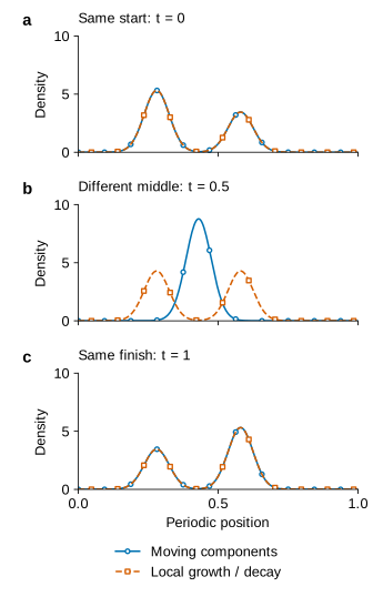
Moving-component and stationary-reaction histories have coincident initial and final densities but visibly different densities halfway through the interval. — Figure 2. Two declared histories for the same swapped-weight endpoint pair, with centres 0.28 and 0.58 and equal endpoint mass. The blue moving-component path and orange stationary growth-and-decay path coincide at times 0 and 1; alternating open markers make the intentional overlap visible. At time 0.5, one concentrates density where the components meet, while the other changes the two stationary peaks. These are known generating paths, not interpolations recovered by the UOT solver. A suitable intermediate observation could distinguish this pair.

For the moving history, $f_{\mathrm{history}}=1$ . For the stationary reaction history, it is zero. Any endpoint-only diagnostic returns the same value $f$ for both histories. Consequently,

\max\{|f-1|,\ |f-0|\}\geq \frac12.

At least one interpretation must be wrong by half a unit or more. This elementary inequality is not a newly discovered limitation of optimal transport; it makes the information deficit explicit for the constructed pair.

The fixed grid contains 360 equal-mass ambiguous fits across geometry, displacement and cost settings. Every one is evaluated against both histories. The smallest observed worst-history discrepancy is approximately 0.50027, consistent with the analytical lower bound. Doubling the number of histories in this comparison does not double the amount of endpoint information.

Nor does the example establish that every ecological inverse problem is impossible. Restricting allowable velocities, measuring reaction, or observing intermediate states may exclude one of the histories. Identifiability is always relative to a model class and an observation system. The failure here concerns endpoints alone when both declared mechanisms remain admissible.

The price of growth changes the explanation

We vary requested displacement over 0, 0.03, 0.06, 0.10 and 0.16; mass ratio over 0.60, 0.80, 1, 1.25 and 1.60; penalty scale over eight values from 0.02 to 0.46; and entropy weight over 0.0025, 0.005 and 0.01. The same endpoint pair is fitted at every relevant cost setting.

These are choices of model and regularization, not repeated noisy samples. The spread across them is a sensitivity analysis. It does not define a confidence interval for an unknown environmental quantity.

$Static transport-cost fractions vary with penalty scale and entropy, compared with the separately calculated generating action fraction for translation, growth and mixed histories.$

Figure 3. Static cost share versus generating action share for the first three examples of Figure 1. Coloured curves are fitted cost fractions at the three stated entropy weights; the black dash-dot line is the independently known dynamic action fraction. All use the 256-cell grid and centres 0.28 and 0.58. Pure translation has true action fraction one; pure growth has zero. For the mixed history, changing the reaction price also changes the true weighted action fraction. Similarity between curves is diagnostic agreement, not proof that the two formulations are equivalent.

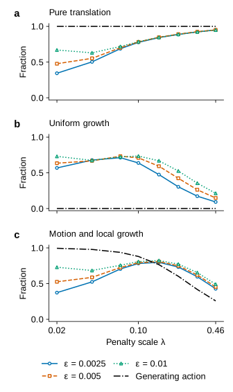
The translation control becomes increasingly transport-dominated as the penalty for marginal change grows. That direction is intuitive: abandoning the correspondence becomes expensive. But at weaker penalties, the cheapest explanation need not pay to move all the mass through the generating displacement.

Uniform growth presents a different problem. Its true kinetic action is zero. Nevertheless, a diffuse regularized coupling can pair nearby but distinct positions and accumulate transport cost. Increasing the marginal penalty does not simply remove every artifact at once, because the marginal adjustment, coupling diffuseness and overall transported mass interact.

The mixed case illustrates why a changing label is not automatically a numerical failure. Both the fitted cost share and the generating weighted action depend on the price assigned to reaction. If a fixed history moves from “transport-dominated” to “mixed” when the price changes, the underlying activity has not necessarily changed. We have changed the accounting rule.

To make label comparisons reproducible, we call a fraction at most 0.25 reaction-dominated, at least 0.75 transport-dominated, and intermediate values mixed. These cutoffs are conventions, not natural constants. We also check 0.20/0.80 and 0.30/0.70. The continuous fractions carry more information than the categories.

Across nontrivial endpoint cases, 364 of 522 penalty-scale sweeps change the fitted label: 69.73%. Across entropy sweeps, 218 of 1,392 do so: 15.66%. The first percentage includes changes in the price of reaction; it should not be described as a pure estimate of numerical instability.

Two heatmaps show absolute disagreement between static cost fraction and known action fraction across penalty scale and displacement or mass ratio; no-change columns are grey and undefined. — Figure 4. Mechanism-interpretation maps for the middle peak geometry at entropy weight 0.005. The upper panel varies requested displacement in pure translation; the lower varies mass ratio in pure growth. Colour records absolute disagreement between static cost share and the known action fraction, on a common zero-to-one scale. Grey cells with dashes are no-change cases: both true action components vanish, so their fraction is undefined, not zero. Requested displacements use their saved nearest-cell realizations in all calculations.

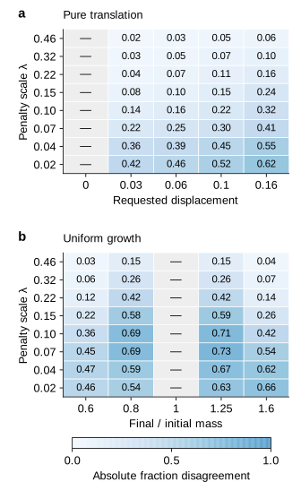
The heatmaps do not identify a universally correct penalty scale. A parameter that improves agreement in one family may worsen it in another. Selecting a scale because it reproduces a desired mechanism would require independent scientific justification. Otherwise, the calibration has quietly supplied the conclusion.

A good fit can answer the wrong question

What should “reconstruction error” mean when the method is allowed to change its marginals? We use the relative L1 discrepancies between the fitted row sums and the initial map, and between the fitted column sums and the final map. A larger value means that the coupling leaves more of the corresponding endpoint unexplained by direct matching.

One could add residual fields back to the coupling and reconstruct both input maps exactly. That bookkeeping identity would not demonstrate successful inference. The original inputs are already available; exact recovery by adding their discrepancies back contains no new information about the unobserved history.

Scatter plots compare the larger endpoint marginal error with mechanism-fraction disagreement in all four families, including separate moving and local-reaction truths for ambiguous endpoints. — Figure 5. Endpoint fidelity and interpretation disagreement at entropy weight 0.005, using all three geometries and all relevant penalty scales. Each point represents one defined history comparison; no-change targets are excluded. The horizontal coordinate is the larger of the two relative marginal L1 errors, expressed as a percentage. In the ambiguous panel, blue circles evaluate the moving history and orange plus signs the stationary reaction history for the same fitted endpoint couplings. Overlapping points are retained; they are not independent observations or uncertainty samples.

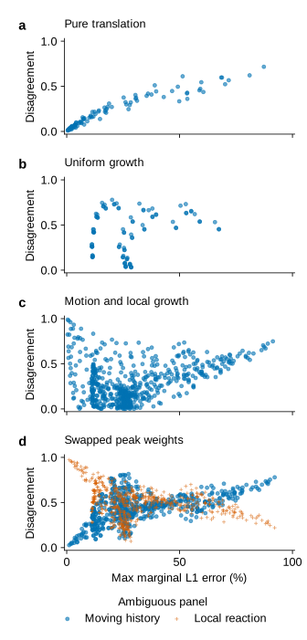
For a concrete example, take the equal-mass swapped-weight pair with centres 0.28 and 0.58, no global shift, $\lambda=0.46$ , and $\varepsilon=0.005$ . Both marginal errors are approximately 3.565%, while the static transport share is 89.14%. That share is much closer to the moving history than to the stationary reaction history. Yet both generated the same observations.

The fit is not fraudulent, and the optimization need not be inaccurate. Its good agreement with the endpoints simply answers a different question. It shows that the chosen coupling is compatible with the maps under the declared penalties. It does not show that the cost-favoured history was the actual one.

As a descriptive check, imposing a 5% ceiling on both marginal errors leaves 221 fitted configurations and 257 defined history comparisons. Of those comparisons, 112 still disagree in fraction by more than 0.25. The 5% cutoff is a reading aid chosen for this summary, not a preregistered success criterion, a statistical confidence level or a general definition of acceptable fit.

This is a useful distinction when interpreting an attractive visualization. Ask whether the arrows have been validated against trajectories, whether the growth map has been checked against a separate measurement, or whether both are merely components of an endpoint discrepancy. Those can all be legitimate outputs, but they justify different sentences.

Why an unchanged map still has a transport cost

Entropy regularization makes a coupling spread its mass across more than the exact diagonal. Pairing a source cell with a nearby destination then contributes positive squared-distance cost, even if the two marginal maps are identical. The marginal penalty can also remain positive because the problem permits marginal relaxation.

The resulting ratio can look dramatically transport-dominated simply because the marginal penalty is even smaller. A fraction close to one says something about relative sizes in its denominator. It does not tell us that the numerator represents a large or physically real activity.

Identical maps produce positive transport, marginal and regularization costs; a second panel shows their static transport fraction approaching one despite a no-change generating history. — Figure 6. A negative control with identical inputs, centres 0.28 and 0.58, and 256 cells. The upper panel separates raw objective contributions at penalty scale 0.10; hatches distinguish marginal and plan KL penalties. The lower panel varies penalty scale for all three entropy weights. The declared physical history is stationary with no reaction, so its action fraction is undefined. At scale 0.46 and entropy 0.005, the static transport share is 99.29%; that number is not a recovered motion fraction.

A standard response to regularization bias is to compare a cross-cost with self-costs. For this precise product-reference objective, the debiased scalar used here is

\begin{aligned} S_\varepsilon(a,b)={}&J(a,b)-\frac12J(a,a)\\ &-\frac12J(b,b)\\ &+\frac{\varepsilon}{2}(M_a-M_b)^2, \end{aligned}

where $M_a$ and $M_b$ are total masses and each $J$ denotes a minimized objective. The mass correction belongs to this formulation; dropping it would change the discrepancy for unequal masses.

This scalar is zero for identical inputs. That is a useful correction to a discrepancy measure. It does not turn the separate transport and growth terms into observed physical actions. Subtracting self-costs component by component can produce signed pieces, and there is no reason to present those pieces as a nonnegative biological budget.

Reducing entropy can make the coupling sharper, but it also changes conditioning and computation. More importantly, the identical-endpoint ambiguity of Figure 2 survives even without regularization. Numerical bias and structural non-identifiability are different problems. Fixing the former cannot, by itself, fix the latter.

What the balanced baseline deliberately forgets

Balanced transport requires equal total mass. Our comparison normalizes each endpoint separately and then solves one entropic balanced problem with the same circular ground cost. It is a shape-only baseline. The normalization is explicit because it removes precisely the information that distinguishes uniform growth from no change.

If $b=ca$ , dividing both maps by their own totals produces the same probability distribution for every positive $c$ . No method receiving only those normalized maps can infer the discarded scalar. This is an information-processing choice made before optimization, not a weakness discovered inside the solver.

Uniformly rescaled density maps become identical after normalization; balanced shape cost stays constant with mass ratio while the unbalanced debiased discrepancy responds to mass change. — Figure 7. What normalization removes, using pure-growth endpoints with centres 0.28 and 0.58. The top two panels show raw and normalized densities at mass ratios 0.60, 1 and 1.60; staggered markers expose intentionally coincident normalized curves. The lower panels cover all five mass ratios. Balanced transport cost uses normalized measures and entropy 0.005; UOT divergence uses raw measures, the same entropy and penalty scale 0.10. The two vertical axes describe different quantities and are not a ranking of method quality. The positive balanced self-cost is regularization-related.

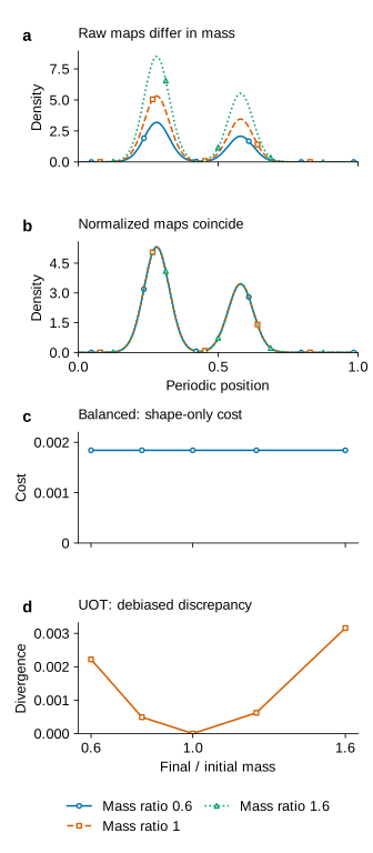
The unbalanced discrepancy remains sensitive to a change in total mass. That makes it useful when both amount and spatial arrangement matter. But detecting that something changed is still different from identifying the mechanism of change. A useful discrepancy need not be a causal reconstruction tool.

Pixelwise L1 and L2 comparisons provide another reference. They faithfully record changes at fixed coordinates, but do not match displaced structure. A small translation of a sharp peak can therefore generate a large difference-map signal. Transport introduces a geometry for comparing such displaced structure. The benefit is real, even when we refuse to interpret the resulting correspondence as a tracked trajectory.

How much of the result is numerical?

The UOT solver is checked against a closed-form single-site solution, independent convex minimization on a small problem, and the established Python Optimal Transport implementation. The single-site check is particularly revealing because every term can be inspected directly:

p^\star=\exp\!\left( \frac{(4\lambda^2+\varepsilon)\log(ab)-C} {8\lambda^2+\varepsilon} \right).

Here $a$ and $b$ are the two scalar masses and $C$ is their transport cost. Agreement tests the mass convention, entropy reference and marginal coefficient together. It would be easy to obtain a plausible matrix while solving a slightly different objective if one of those conventions were changed silently.

At the main grid size, selected full matrices agree with the independent implementation to relative L1 differences below $7.0\times10^{-7}$ . Tightening solver tolerances changes the selected cost fractions by less than $1.9\times10^{-7}$ . Repeated selected solves are identical in the recorded environment. These checks address implementation and numerical precision, not identifiability.

Grid refinement uses matched physical displacements rather than rounded shifts that differ across grids. The largest selected change from 256 to 512 cells is below $4.8\times10^{-8}$ in cost fraction. One coarser 128-cell comparison exceeds the stricter refinement threshold; further checking at 1,024 cells supports the main-grid result. That coarse-grid exception is retained rather than folded into a statement that every check passed.

Empirical timing curves compare 180 matched UOT and balanced configurations; a residual-versus-iterations plot retains the balanced solver cases that reach the iteration cap. — Figure 8. Computational behaviour on this host, not a portable speed benchmark. The upper panel uses the same 180 labelled endpoint cases for both solvers, entropy 0.005 and UOT scale 0.10; each time is measured once. Crosses mark balanced solves reaching the iteration cap. The lower panel includes all 540 balanced fits across the three entropy values, with a dotted residual threshold of 10⁻⁹. Fourteen reach 20,000 iterations without meeting it. Some coincide because normalization makes multiple growth cases identical. Failed costs are retained as failures, not accepted baseline solutions.

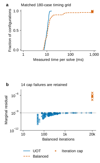
Across the complete recorded grids, median solve times are 10.74 ms for UOT and 10.99 ms for the balanced baseline. Those summaries weight parameter configurations differently, so the matched comparison in Figure 8 is the more informative visual reference. Neither supports a universal claim that one method is faster.

All 4,320 main UOT fits and 4,248 cached self-cost fits meet the declared criteria. Fourteen of 540 balanced fits do not converge within the fixed cap. An independent implementation reproduces slow convergence for a separated-peak example under the same cap. We do not silently raise the cap, loosen the tolerance, or replace those entries with seemingly successful costs.

This matters scientifically because a failed solver and a non-identifiable mechanism demand different responses. A failed solver calls for numerical investigation. An endpoint ambiguity calls for additional information or narrower assumptions. Treating both as “the model needs more training” would obscure the difference.

What would make a physical explanation more credible?

The middle panel of Figure 2 suggests the most direct experiment: observe the system between the two endpoints. The two constructed histories have different intermediate shapes, so a suitably timed and resolved observation could distinguish them. A noisy or heavily aggregated observation may not; the information gain depends on what the sensor actually measures.

An intermediate total can also matter here because the stationary reaction path need not preserve total mass throughout the interval. But this is a property of this pair, not a theorem that three total measurements identify an arbitrary velocity and reaction field. More complicated histories could match the additional measurement too.

Independent constraints on reaction offer another route. If known growth rates cannot generate the observed change over the available time, the admissible reaction-only explanation shrinks. Conversely, velocity observations or a physical upper bound on travel distance can exclude implausibly rapid transport. Such information should enter as a stated assumption or observation, not as a penalty tuned until the arrows look convincing.

Tracking labelled material is stronger still. A correspondence between density maps does not reveal individual identities. Tracers, particles or identifiable objects may supply that missing link. They also bring their own sampling biases and detection errors, so a complete analysis would propagate those uncertainties rather than simply declaring the trajectory known.

There is a practical sequence here. First define the field and its units. Then specify the histories considered physically admissible. Next ask which observations would separate competing histories. Only after that should an optimizer be chosen to summarize or estimate within the constrained problem. Starting with an attractive optimizer and interpreting every output term physically reverses that sequence.

The next scientifically useful step is therefore not automatically a larger neural model. For this controlled problem, it is an explicitly designed additional-observation experiment: add one intermediate map or a measured reaction constraint and test which ambiguities remain. That is a different study, not a result already obtained by the present endpoint-only benchmark.

Where this sits in the literature

Unbalanced transport and Wasserstein–Fisher–Rao geometry already provide mature mathematical languages for movement and mass variation. Their applications to reaction–advection–diffusion models and biological flows are substantial. Entropic scaling, debiased discrepancies, accelerated dual methods, constrained geodesics and scalable decomposition solvers address different aspects of this established field.

The closest practical overlap is Francis, Cotter and Mittermaier’s work on entropic unbalanced transport for spatial forecast verification. It already examines spatial perturbations, mass differences, parameter scales and cost decomposition. Our parameter-sensitivity plots should not be presented as the invention of that idea.

Ponnoprat, Isobe and Imaizumi’s 2026 preprint studies estimation of transport–growth pairs defined by a UOT oracle. That target is not an arbitrary history chosen to generate the data. Recovering an optimal pair accurately and proving that it equals the historical physical mechanism are different tasks.

Recent WFR-FM, published at ICLR 2026, and the WFR-MFM preprint concern learned flow-matching constructions in WFR-related geometries. They are relevant context, but no neural flow matching is used here. A method designed to represent or approximate a chosen geometric path does not, by that fact alone, resolve the endpoint ambiguity exhibited above.

The contribution of this article is consequently modest: a verified synthetic comparison and a reader-facing examination of a tempting interpretation. It does not establish priority for an identifiability theorem, propose a new solver, or validate a field application.

Conclusion

Two maps can support a useful distance, a useful correspondence, and a useful least-cost explanation without identifying what happened between them. Those are not contradictory statements. They describe different levels of inference.

In this benchmark, the numerical optimization is often precise while the physical interpretation remains fragile. Cost shares change with prices and regularization. Identical maps can have positive raw transport cost. Most decisively, a moving history and a stationary reaction history can present exactly the same endpoint evidence.

The right question is therefore not only “Does the coupling fit?” It is “What information would rule out the competing history?” Until that question is answered, an unbalanced transport decomposition is an explanation selected by a model—not a witnessed account of how the hotspot changed.

References

Chizat, L., Peyré, G., Schmitzer, B. and Vialard, F.-X. Unbalanced Optimal Transport: Dynamic and Kantorovich Formulations. Journal of Functional Analysis, 2018. Original research.
Liero, M., Mielke, A. and Savaré, G. Optimal Entropy-Transport Problems and a New Hellinger–Kantorovich Distance between Positive Measures. Inventiones Mathematicae, 2018. Original research.
Liero, M., Mielke, A. and Savaré, G. Optimal Transport in Competition with Reaction: The Hellinger–Kantorovich Distance and Geodesic Curves. SIAM Journal on Mathematical Analysis, 2016. Original research.
Cuturi, M. Sinkhorn Distances: Lightspeed Computation of Optimal Transport. NeurIPS, 2013. Proceedings paper.
Chizat, L., Peyré, G., Schmitzer, B. and Vialard, F.-X. Scaling Algorithms for Unbalanced Optimal Transport Problems. Mathematics of Computation, 2018. Original research.
Séjourné, T., Feydy, J., Vialard, F.-X., Trouvé, A. and Peyré, G. Sinkhorn Divergences for Unbalanced Optimal Transport. Author preprint.
Séjourné, T., Vialard, F.-X. and Peyré, G. Faster Unbalanced Optimal Transport: Translation Invariant Sinkhorn and 1-D Frank–Wolfe. AISTATS, 2022. Proceedings paper.
Gallouët, T. O., Laborde, M. and Monsaingeon, L. An Unbalanced Optimal Transport Splitting Scheme for General Advection–Reaction–Diffusion Problems. ESAIM: Control, Optimisation and Calculus of Variations, 2019. Publisher paper.
Francis, J. J. M., Cotter, C. J. and Mittermaier, M. P. Examining Entropic Unbalanced Optimal Transport and Sinkhorn Divergences for Spatial Forecast Verification. Meteorological Applications, 2025. Author full text.
Bauer, M., Charon, N., Needham, T. and Nishino, M. Path Constrained Unbalanced Optimal Transport. Nonlinearity, 2025. Author full text.
Medina, I., Nguyen, T. S. and Schmitzer, B. Domain Decomposition for Entropic Unbalanced Optimal Transport. Computational Optimization and Applications, 2026. Publisher article.
Ponnoprat, D., Isobe, N. and Imaizumi, M. Minimax Optimal Estimation of Transport-Growth Pairs in Unbalanced Optimal Transport. 2026 preprint. Author full text.
Peng, Q. and colleagues. WFR-FM: Simulation-Free Dynamic Unbalanced Optimal Transport. ICLR, 2026. Official proceedings.
Wang, X. and colleagues. WFR-MFM: One-Step Inference for Dynamic Unbalanced Optimal Transport. 2026 preprint. Author full text.