If You Only Observe Aggregates, Can You Still Bound the Hidden Epidemic?

A dashboard reports a total of infected people across several neighbouring regions. The number is a little old, and the measurement is imperfect. Behind that one number, one region might be recovering while another is still growing. A filtering algorithm supplies six smooth curves and a narrow shaded band around each. The display looks reassuringly specific.

What, exactly, has become specific? Has the data excluded every substantially different regional trajectory? Or has the algorithm selected a small set of trajectories that fit its probability model particularly well?

Those are different accomplishments. This article investigates the difference in a hypothetical six-region epidemic. There are no patient records, fitted disease parameters or claims about a current outbreak. Every observation is generated from a known synthetic model. That controlled setting lets us inspect the hidden truth and ask whether two very different kinds of uncertainty interval actually contain it.

The first method is an ensemble Kalman filter, or EnKF. It uses a population of simulated states to estimate how observations and hidden variables move together. The second is set-membership estimation: keep every state that has not been excluded by the declared initial conditions, model and error limits, using a computable outer enclosure when the exact set is too complicated.

The important word is outer. An enclosure can retain the truth while retaining far too many other possibilities. A mathematical containment argument is not a promise that its answer will be useful. Conversely, a narrow ensemble interval can be valuable without being a deterministic bound. The project overview gives the short version; here we work through the mechanisms, eight figures and limitations.

What the comparison found

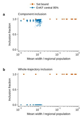
The two-group, five-day-delay baseline gives the central tension. Across 50 replicates, the set enclosure spans an average 48.40% of regional population, against 0.951% for EnKF. The set retains every complete infected trajectory; the EnKF retains none completely, although its component inclusion averages 94.05%. These are different measures of reliability, not a contradiction.

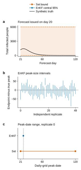
Once observations stop after the day-20 forecast, the set’s baseline peak-size range becomes 0–6,000, with candidate dates spanning 21–120. Containment survives, but precision largely disappears. The study therefore does not crown a universal winner: it separates distributional usefulness, conditional protection and algorithmic conservatism.

A total is a measurement, not a regional map

The observed quantity is the number currently infected, not the number of new infections during a day. This distinction determines the measurement equation. An infected stock is a state at a particular time. Daily incidence counts transitions into that state over an interval. Recovery, movement and the timing of reporting make the two quantities different even in a perfectly measured model.

Our six regions begin with populations of 1,000, 900, 1,100, 950, 1,050 and 1,000. Initial infected counts are centred on 8, 5, 6, 4, 7 and 5, with each allowed to vary independently by two people in either direction. Nobody has recovered initially. The remaining people are susceptible. These counts are continuous model quantities; fractional people later in a trajectory represent the approximation built into a compartmental differential equation, not partially infected individuals.

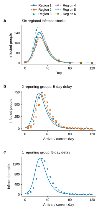
We compare three reporting arrangements. Six groups report each region separately. Two groups report regions 1–3 and 4–6. One group reports the total across all six. In every arrangement, a report is the sum of the relevant infected states plus an error whose absolute magnitude is bounded.

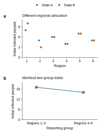
Six synthetic regional infection curves followed by two-group and one-group totals, with delayed observations plotted at their arrival dates. — Figure 1. What is observed in preselected replicate 0 of the six-region SIR experiment. The top panel separates the six true infected stocks; the lower panels combine them into two groups or one. In the two-group panel, blue circles represent regions 1–3 and orange squares regions 4–6. Lines show current truth, while open markers show five-day-delayed reports with error bounded by five people per group. For legibility, only every fifth received report is marked; the algorithms use every daily report. Baseline process bound is 0.5 and movement rate is 0.002 per day.

Suppose the first group contains 19 infected people. The vectors (8, 5, 6) and (10, 3, 6) give the same total. This example stays inside the declared initial uncertainty range. The second regional distribution is not a fabricated estimate produced by the filter; it is an alternative admissible initial state used to illustrate the measurement map. Its susceptible counts change in the opposite direction, so each initial regional population is preserved.

One sum has discarded the direction that transfers infection from one member of the group to another while keeping the group total fixed. If that sum were all we could ever learn, the ambiguity would be unavoidable. But the experiment supplies a sequence of observations, and regions have different infection rates. Their future totals can therefore respond differently to the two initial distributions.

That qualification matters. An ambiguous snapshot is not a proof that the entire dynamical system is unobservable. Time evolution may reveal information that a single observation cannot. We have not established a global impossibility theorem for this six-region model. Instead, the benchmark asks what two particular algorithms do with a limited sequence of noisy, delayed aggregates.

Two admissible initial infection allocations differ in regions one and two but have exactly coincident totals within both reporting groups. — Figure 2. An exact single-time ambiguity, not a Monte Carlo result. State A has infected counts (8,5,6,4,7,5); state B transfers two infections from region 2 to region 1. Both respect the initial bounds, with opposite susceptible adjustments preserving population. Their two-group totals are exactly equal. Open squares and filled circles deliberately coincide in the lower panel; small horizontal offsets in the upper panel only separate the categorical markers. No claim about identical future observation sequences follows.

Notice another fairness detail. The measurement error limit is attached to each reported group, not each underlying person or region. A one-group total has one bounded error; summing six separate reports would combine six errors. Thus the reporting arrangements are different information systems, not a cost-matched sensor-placement experiment. Moving between them changes both regional resolution and the way errors enter the totals. We should not turn their ranking into an economic recommendation about purchasing sensors.

People move, so the denominators move too

Each region has susceptible, infected and recovered compartments, denoted by $S_i$ , $I_i$ and $R_i$ . Its population is their sum, $N_i=S_i+I_i+R_i$ . Regions form a ring: people move to either neighbouring region at the same per-person rate. The neighbours of region 1 are regions 2 and 6. The same movement rule applies to all three compartments.

Between the daily disturbances, the model is

\begin{aligned} \mathcal M_i(Z)&=m(Z_{i-1}+Z_{i+1}-2Z_i),\\ \dot S_i&=-\beta_i\frac{S_iI_i}{N_i}+\mathcal M_i(S),\\ \dot I_i&=\beta_i\frac{S_iI_i}{N_i}-\gamma I_i+\mathcal M_i(I),\\ \dot R_i&=\gamma I_i+\mathcal M_i(R). \end{aligned}

The infection rates are $(0.36,0.34,0.38,0.33,0.35,0.37)$ per day, and the recovery rate is $0.14$ per day. The baseline movement rate to each neighbour is $0.002$ per day. These are fixed synthetic inputs, not estimates of any disease. No unknown parameter is fitted during filtering.

Adding the three equations removes infection and recovery, leaving a movement equation for population:

\begin{aligned} \dot N_i&=m(N_{i-1}+N_{i+1}-2N_i),\\ \sum_{i=1}^{6}N_i(t)&=6000. \end{aligned}

The total population is constant. Each regional population generally is not. Replacing every denominator by its initial population would silently change the model. For this symmetric ring, movement averages neighbouring populations: the largest cannot increase and the smallest cannot decrease. Consequently, every regional population stays between 900 and 1,100. This physical constraint also keeps the infection denominators away from zero.

After each completed day of continuous evolution, a bounded disturbance transfers people between susceptible and infected compartments in the same region. A proposed transfer is clipped only when necessary to avoid a negative compartment. In the baseline, its magnitude is at most half a person per region per day. It can increase or decrease infection; it is a deliberately simple discrepancy model, not a literal description of a particular epidemiological mechanism.

\begin{aligned} u_{i,n}&=\operatorname{clip}\bigl(\widetilde u_{i,n},-I_i(n^-),S_i(n^-)\bigr),\\ S_i(n)&=S_i(n^-)-u_{i,n},\\ I_i(n)&=I_i(n^-)+u_{i,n},\\ R_i(n)&=R_i(n^-). \end{aligned}

Here $n^-$ means just before the daily transfer. The proposed transfer satisfies $|\widetilde u_{i,n}|\le q$ , with baseline $q=0.5$ . This operation preserves each regional population. The observation is then taken from the post-transfer state. The order is continuous evolution, bounded transfer, measurement, followed by any reporting delay.

Writing that sequence explicitly avoids a surprisingly consequential ambiguity. Adding independent perturbations to all compartments would not preserve population. Treating a daily bounded transfer as continuous white noise would specify a different uncertainty model. Allowing fresh arbitrary disturbances at every numerical substep would increase the total disturbance budget when the solver took smaller steps. None of those alternatives is used here.

Near a boundary, clipping also changes the realised disturbance distribution. If infection is almost zero, a proposed negative transfer cannot remove more infected people than exist, whereas a positive transfer can still introduce infection from the susceptible compartment. A symmetric proposed error therefore need not have a zero-mean realised effect. Both truth and ensemble apply the same rule; the set method encloses every allowed clipped transfer. Any late synthetic infection supported by this mechanism is not evidence of observed reinfection or external importation.

A report has two dates

A report is labelled by the day it measures and the day it becomes available. With a five-day delay, a report arriving on day 20 measures infection on day 15. Its error bound is about the day-15 total. It is not a five-day-old approximation that can safely be attached to the day-20 state.

For a grouping matrix $C$ , the observation equation is

\begin{aligned} y_n&=C I(n)+v_n,\qquad |v_{g,n}|\le\bar v,\\ \text{arrival day}&=n+d. \end{aligned}

Every row of $C$ contains ones for its member regions and zeros elsewhere. The delay $d$ is known and restricted to whole days. We examine 0, 5 and 10 days. A fractional delay is rejected, not rounded down to the nearest observation. There are no invented pre-study measurements: before the first report arrives, an estimator has only its initial information and model.

Both algorithms maintain their updated state at the latest measured day. When the next report arrives, they advance that historical state by one day, apply its measurement update, and then propagate forward across the known delay to produce a current estimate. The forward prediction uses only the model and allowed disturbances. It does not use observations that will arrive tomorrow.

This is more than bookkeeping. In a growing phase, applying an old, smaller total directly to today’s state would bias an update downward. In a declining phase, the same shortcut could bias it upward. A narrow band produced by such a mistake would be a timing error masquerading as precision. The comparison therefore shares both the observations and their availability schedule.

Delayed updating also changes computational work. A ten-day delay requires repeated forward propagation to answer today’s question after each historical update. The historical posterior and today’s prediction are not the same object. Any claim that one method is faster must state whether it includes that extra propagation. Our filtering timing includes it; the separate long-range peak forecast is not included in that timing.

What the ensemble learns from its members

An EnKF begins with many possible states. Here there are 500 members in the main comparison. Each starts from an independent draw within the same initial infection bounds as the truth. Each undergoes its own bounded, population-preserving daily transfers. Across members, the distribution shows how the assumed prior and process model spread uncertainty through time.

When a report arrives, each member predicts the corresponding regional sums. If members with larger group totals also tend to have larger infection in region 2, that covariance gives the filter a route from a measured sum to an unmeasured regional state. It is useful information, but it comes partly from the ensemble’s distribution and dynamics, not only from the latest total.

The analysis update has the familiar form

\begin{aligned} K&=P_{xy}(P_{yy}+R_v)^{-1},\\ x^{a,(j)}&=x^{f,(j)}\\ &\quad+K\bigl(y+\varepsilon^{(j)}-C I^{f,(j)}\bigr),\\ R_v&=\frac{\bar v^2}{3}\,\mathrm{Id}. \end{aligned}

The matrices $P_{xy}$ and $P_{yy}$ are sample covariances across members. The superscripts distinguish forecast and analysis states. Observation errors and the artificial observation perturbations are sampled uniformly on $[-\bar v,\bar v]$ , independently across groups. That uniform distribution has variance $\bar v^2/3$ ; using $\bar v^2$ as its variance would compare a different filter. Initial and proposed process errors are also sampled uniformly inside their specified bounds.

The linear update can produce nonphysical states. We therefore project each member’s three compartments in each region onto the nonnegative simplex whose sum is that region’s independently evolved population. This projection is the Euclidean nearest physical state under that constraint. It is a declared part of the implementation, not an after-the-fact deletion of awkward members.

There is no covariance inflation or localisation in this benchmark. That keeps the comparison fixed and inspectable, but it also limits the conclusion: the result describes this EnKF configuration, not the best possible tuned ensemble method. Changing the ensemble size tests sampling sensitivity; it does not explore every calibration technique.

The displayed EnKF bands are the 2.5th and 97.5th percentiles of each infected component across members. They are central 95% ensemble intervals. They are not exact Bayesian credible intervals in this nonlinear, projected filtering scheme, and they are not deterministic enclosures of all states allowed by the error bounds. A member population represents a distribution; even an ideal central interval deliberately leaves some probability in its tails.

There is a second distinction between a component interval and a whole trajectory. An interval that contains region 2 on day 15 can miss region 4 on day 38. Keeping every region inside on every day is a much more demanding event. Reporting only the average fraction of covered region-days would conceal that difference. We measure both, without pretending that the 720 region-day checks in a run are independent experiments.

What a set bound refuses to discard

Set-membership estimation asks a different question: which states remain possible if the model and all declared error limits are correct? It does not require a probability density within those limits. A disturbance near the edge is retained just as seriously as one near the centre. The uniform distributions used to generate the benchmark are not needed for the set-containment argument.

Exact feasible sets quickly become complicated. Nonlinear dynamics bend them; repeated observations cut them; movement couples regions. We use a simple computational representation: a box giving a lower and upper endpoint for each compartment, together with nonnegativity and population constraints. This is intentionally a conservative baseline, not a claim that boxes are the most efficient set representation.

If a group total lies between $a$ and $b$ , a regional infected component must obey

I_j\ge a-\sum_{i\ne j}U_i,\qquad I_j\le b-\sum_{i\ne j}L_i.

The sums here run over the other regions in that group. Intersecting these limits with the existing component interval cannot remove a state that satisfies the group constraint. The same idea contracts compartments using $S_i+I_i+R_i=N_i$ and contracts populations using the total of 6,000. Repeating the contractions can improve them, although a fixed number of passes need not recover the tightest possible box.

The logic is elementary but revealing. A total of 19 is informative about region 1 only to the extent that the possible contributions of the other regions are restricted. Wide uncertainty elsewhere leaves room to exchange infection between regions. The resulting bounds express an inability to eliminate alternatives, not a statement that all alternatives are equally probable.

Propagation between measurements needs more care. Integrating the lower corner and upper corner separately does not generally bound a nonlinear epidemic model. The dynamics can couple variables with opposing effects. Sampling many trajectories also cannot establish that no unsampled admissible trajectory escapes.

Instead, each numerical step constructs a tube $Y$ around the current box $B$ . Interval arithmetic evaluates a range $F(Y)$ that contains the vector field over the tube’s physical domain. A step of length $h$ is accepted only when

\begin{aligned} B+[0,h]F(Y)&\subset\operatorname{int}(Y),\\ B_{\mathrm{next}}&\subseteq B+hF(Y). \end{aligned}

The second expression means the computed next box is obtained by intersecting the outward-rounded endpoint enclosure with known physical constraints. The containment claim is about feasible trajectories, not arbitrary points removed by those constraints. The strict tube test supplies the important argument: if a physical trajectory tried to leave the tube for the first time, its accumulated derivative would still put it strictly inside. That contradiction keeps the trajectory in the tube for the whole step.

The endpoint enclosure then includes the integral of every derivative the trajectory could encounter. This is a first-order range enclosure, not ordinary Euler stepping with a missing truncation-error term. Its price is width. By replacing the changing derivative with an interval range, it loses temporal and cross-variable dependencies that a high-order validated method might preserve.

All elementary interval additions, subtractions, multiplications and divisions are rounded outward under finite IEEE 754 double-precision arithmetic. Sums use explicitly rounded additions. Positive denominators are checked. The nominal interval step is a quarter of a day; a failed tube test triggers subdivision, and failure at the minimum permitted step returns a validation error rather than an unchecked result.

The daily disturbance is enclosed by adding its allowed range to susceptible and infected components, then contracting with physical constraints. This forgets that their changes are opposite. Forgetting that correlation enlarges the set; it does not justify shrinking it. Such repeated losses of dependency are a major source of conservatism in the later figures.

The complete conditional argument therefore follows the actual computation: the initial set contains the allowed starts; a validated step preserves containment; the bounded transfer preserves it; the correct historical measurement strip preserves it; and forward propagation through the delay preserves it. An empty intersection is reported as empty. It is not repaired by quietly widening the observation error or restarting from the truth.

Measuring usefulness without counting the same experiment twice

The main design crosses three grouping arrangements, three delays and two measurement-error bounds: 6, 2 or 1 groups; 0, 5 or 10 days; and 1 or 5 people per report. That gives 18 settings, each with 50 independent replicates. Four additional settings change one feature of the two-group, five-day, five-person baseline: the process bound becomes 0 or 1, or the movement rate becomes 0 or 0.01. The main and sensitivity experiments therefore contain 1,100 complete 120-day replicate runs.

The methods see paired data within every replicate. Separate random streams supply initial truth, process disturbances, measurements and ensemble members. Compatible settings reuse underlying random draws so that a comparison is not needlessly dominated by different initial epidemics. The statistical unit remains the independently generated replicate, not an individual day, region or ensemble member.

Component coverage averages the inclusion indicators over six infected states and days 1–120 within each run. Simultaneous trajectory coverage is one only if all those checks succeed. Width is divided by the actual, time-varying regional population before averaging:

w=\frac{1}{720}\sum_{n=1}^{120}\sum_{i=1}^{6}\frac{U_i(n)-L_i(n)}{N_i(n)}.

A normalised width of 0.5 means the average component interval spans half of its region’s population. It does not mean a 50% probability of infection. Nor does average width describe every day equally well: a band can be narrow after direct observations and almost unrestricted after a long forecast.

Intervals around reported replicate means use 2,000 percentile-bootstrap resamples of whole replicates. Method differences use paired resampling. This retains each run’s temporal and spatial dependence. When all 50 runs succeed, the ordinary empirical bootstrap returns an interval at one; that is a feature of the resampling calculation, not proof that the population success probability is exactly one. The deterministic set claim, where applicable, comes from the separate inclusion argument.

Timing is measured as wall-clock filtering work divided by the number of replicates and updates in a vectorised batch. It includes delayed current-state propagation. It is an amortised throughput measure on this implementation, not the latency of an isolated live case. Since the batch shares one clock measurement, we do not manufacture 50 independent timing observations or bootstrap a spurious timing confidence interval.

The reference simulation uses high-accuracy adaptive integration, independently compared against a tighter tolerance. Ensemble propagation uses fourth-order Runge–Kutta with a quarter-day step and is checked against a half-sized step. These convergence checks address numerical approximation; they do not convert an ensemble percentile into a guarantee or validate the synthetic model against real disease data.

What the hidden-state intervals actually look like

Direct, current regional reports keep the simple set representation relatively tight. With a five-person measurement bound, increasing delay alone produces the following widths; all entries are percentages of changing regional population, averaged over 50 replicates:

Delay with six reporting groups	Set width (%)	EnKF width (%)
0 days	0.717	0.268
5 days	8.424	0.378
10 days	26.527	0.536

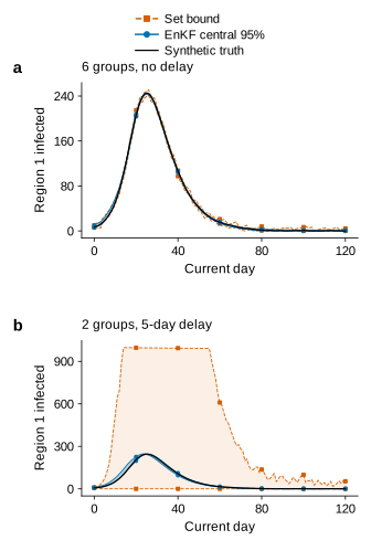
The large increase for the set method is not entirely fresh uncertainty in the physical epidemic. Every unobserved step also loses dependencies in the first-order box representation. Replacing six reports with two grouped totals at five-day delay raises its mean width further, to 48.40%. Figure 3 shows how that difference develops in one preselected trajectory; Figures 4–5 retain the broader comparison.

Nor should a whole-path failure be mistaken for a useless component estimate. Across these three six-group cases, EnKF component inclusion is approximately 94.53%, 95.09% and 95.21%, respectively, while none of the 50 trajectories in each case stays inside every component interval on every day. The mean inclusion is not always below 95%. A demand for simultaneous protection needs a simultaneous uncertainty construction, not a new interpretation of marginal percentiles.

The matched ten-replicate ensemble-size check gives component inclusion of 90.03%, 92.67% and 92.50% for 100, 500 and 1,000 members in the two-group baseline. More members reduce one source of sampling uncertainty but do not guarantee monotone improvement of coverage. These ten runs are a sensitivity subset, not a replacement for the 50-replicate primary estimate.

Region one truth compared with an orange set enclosure and blue central ensemble interval under direct reporting and under aggregation with a five-day delay. — Figure 3. Region 1 in preselected replicate 0, with five-person measurement error, process bound 0.5 and movement rate 0.002 per day. The upper panel receives six direct reports without delay; the lower receives two grouped reports delayed five days. Black is synthetic truth, dashed orange bounds a constrained outer set, and solid blue encloses the central 95% of 500 ensemble members. Shading is not a confidence interval for mean performance. The vertical scales differ so neither scenario is visually flattened.

All primary replicate coverage and width results, separating component inclusion from the stricter event that every region and day is contained. — Figure 4. All 900 primary replicate summaries per method: 18 settings with 50 repeats each. Horizontal position is mean interval width divided by changing regional population, on a logarithmic scale. Vertical position shows component inclusion above and whole-trajectory inclusion below over days 1–120. Squares denote the set method and circles the 500-member EnKF. Values are not displaced to avoid overlap; many exact coincidences, especially zero or one path scores, are intentional. Neither region-days nor members are counted as independent replicates.

Four labelled matrices separate each method's mean normalized width and component inclusion across three grouping resolutions and three reporting delays. — Figure 5. Grouping and delay at the five-person measurement-error bound, baseline process bound 0.5 and movement rate 0.002 per day. Each cell is a mean over 50 independent replicates. The first two panels report normalised width; the next two report component inclusion. Printed numbers carry the quantitative comparison; pale backgrounds are only a reading aid. A cell with inclusion 1.000 records this finite experiment, not a statistical proof of universal success. The one-person cases remain in Figure 4 and the underlying comparison.

Amortized filtering times and paired one-factor sensitivity to daily process bounds and movement, with width and inclusion shown separately. — Figure 6. Top: observed filtering throughput for two groups and five-person measurement error, including propagation across the reporting delay. Times pool batches of ten and are not single-case latency estimates; no timing error bars are invented. Lower panels: baseline versus one-factor process bounds q=0 or 1 and movement rates m=0 or 0.01, all at five-day delay, with 50 replicates each. Top and middle vertical axes are logarithmic. Bars are 95% percentile-bootstrap intervals from 2,000 replicate resamples. Changing q changes both simulated disturbances and the admitted uncertainty, not just an estimator tuning parameter.

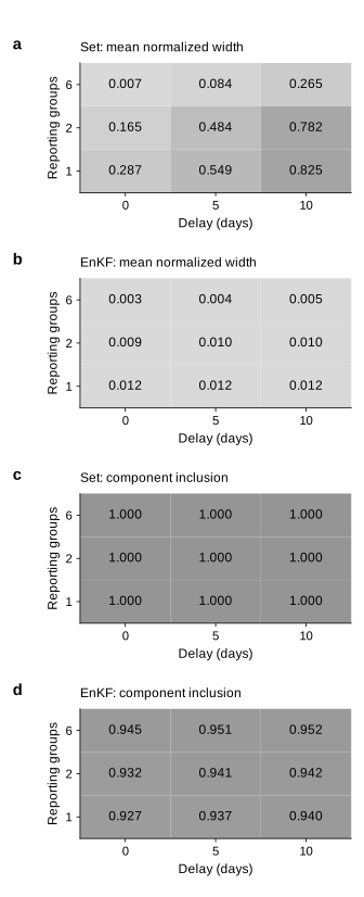
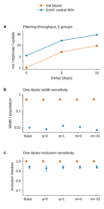
Turning off process disturbance does not rescue this box representation. In the same grouped, delayed setting with q=0, its mean normalised width remains 47.64%, only modestly below the baseline 48.40%. Initial uncertainty, delayed aggregation and lost dependencies are sufficient to keep it broad. This comparison changes the admitted disturbance and generated truth together; it does not show what happens when an estimator wrongly ignores a real disturbance.

The width penalty is also distinct from a time penalty. The recorded baseline throughput is approximately 5.0 ms per replicate-update for the set implementation and 15.7 ms for EnKF. Here the much narrower output costs more computation. These are pooled batch timings under the workload of this run, not isolated latency measurements or a hardware-independent ranking. More elaborate set representations might change both width and cost.

A future peak is a different question

At day 20, we freeze the information available to each estimator and issue one forecast. No later report is assimilated into it. With a ten-day delay, the latest received observation measures day 10. This makes the forecast a genuine test of what can be inferred then, not a retrospectively smoothed estimate that benefits from seeing the peak first.

The forecast concerns total infected people on the daily grid from day 21 through day 120. If its lower and upper envelopes are $L_n$ and $U_n$ , the peak-size enclosure and candidate peak dates follow directly:

\begin{gathered} \max_n L_n\le\max_n\sum_i I_i(n)\le\max_n U_n,\\ \mathcal D=\{n:U_n\ge\max_s L_s\}. \end{gathered}

Every genuine maximising day must belong to $\mathcal D$ : its upper bound cannot fall below a value already forced at some other day. The candidate set can be disconnected. For a compact plot we show its earliest and latest dates, while coverage is checked against the full saved candidate set. The hull can contain dates that the original set excluded; it is an outer summary, not evidence of a continuous plateau.

The total-infection envelope also retains global conservation. It cannot exceed 6,000, and susceptible and recovered lower bounds can reduce that ceiling further. Simply adding six component upper endpoints would forget that their maxima need not occur together. Applying the known sum constraint to the derived total is mathematically different from trimming a plot because it looks too wide.

For EnKF, each member generates a complete future trajectory. We compute its total-infection peak and maximising day first, and only then take central percentiles across members. Taking the maximum of pointwise percentile curves would answer a different question. All reported dates refer to the daily grid; no between-day maximum or exact continuous-time peak date is claimed.

Percentile interpolation can give an ensemble date endpoint between two integers. That is a numerical summary of a distribution of integer dates, not sub-day timing information. Likewise, many members can peak on the same day and produce a zero-width date interval while disagreeing about peak size. Such apparent date precision must be evaluated against the held-out future truth, rather than inferred from the narrowness of the date interval itself.

In the two-group baseline, all 50 set forecasts retain the full 0–6,000 peak-size interval and the 21–120 date span. The EnKF peak-size intervals contain truth in 49 of 50 runs; its date intervals contain truth in all 50. Their mean widths are about 53.06 people and 0.44 days. In replicate 0, the true daily-grid peak is 1,424.32 people on day 26; the ensemble date interval is also day 26. That favourable result belongs to this fixed synthetic model, not to epidemic forecasting in general.

Day twenty forecast with a broad total-infection enclosure, ensemble peak-size errors across fifty replicates, and very different daily-grid peak-date ranges. — Figure 7. Two groups, five-day delay, five-person measurement bound and baseline dynamics. The forecast is issued on day 20 using only reports then received; no later measurements are assimilated. Top: replicate 0 truth and set total-infection envelope on days 21–120. Middle: all 50 EnKF peak-size intervals after subtracting each replicate's true peak; segments that miss zero miss truth. Bottom: replicate 0 peak-date ranges, with a dotted line at its true daily-grid peak. The set's displayed date range is the hull of its retained candidate dates.

When a bound is wrong, empty, or merely unhelpful

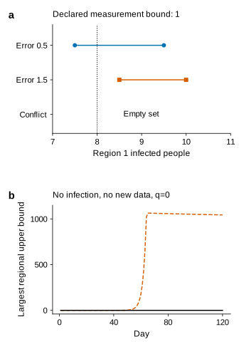
Three failure modes deserve different names. First, a wrong error assumption can give a nonempty set that excludes truth. In the one-step example below, region 1 truly has eight infected people. An error of 0.5 with declared bound one leaves the interval [7.5,9.5]. An actual error of 1.5, still analysed under bound one, gives [8.5,10]: a plausible-looking, nonempty answer that misses eight. Nonemptiness does not validate the assumptions.

Second, conflicting reports can make the intersection empty. Applying a second report offset by ten people to the already constrained state produces that outcome. The implementation reports the contradiction rather than changing its noise allowance. An empty set says the adopted constraints cannot all hold; it does not, by itself, identify which sensor, model term or initial assumption is wrong.

Third, the arithmetic can remain valid while the representation becomes unhelpful. A supplementary analytic control starts with zero infection, zero recovered population and zero process disturbance. True infection stays exactly zero as susceptible people move. Without new observations, the padded first-order boxes nevertheless expand until the largest regional infection upper bound reaches about 1,063.63. Tiny positive ranges admitted by the tube construction are repeatedly propagated and lose dependence. This is a limitation of the implemented enclosure, not evidence that the disease-free system is unknowable.

Valid and mismatched observation bounds for a truth of eight infections, an explicit empty-set outcome, and widening boxes around an exactly disease-free trajectory. — Figure 8. Separate diagnostic examples, not additional primary replicates. Top: region 1 truth is eight, the declared error bound is one, and errors of 0.5 and 1.5 produce different retained intervals. A subsequent report shifted by ten produces an empty set; no interval is drawn for it. Bottom: an exact disease-free control with q=0, baseline movement and no observations for 120 days. The black zero line is truth; the dashed curve is the largest regional box upper bound. No confidence interval or real-outbreak interpretation is attached.

What the literature changes about the conclusion

Interval estimation for epidemics is not new. Aronna and Bliman developed a SIR–SI interval observer under stated model and measurement assumptions. Work by Gouzé and colleagues established interval observers for uncertain biological systems much earlier. These precedents rule out treating the general idea of bounding a hidden epidemic as a new contribution. Their constructions and assumptions are not identical to our hybrid six-region box baseline. SIR–SI interval observer, biological interval observers.

There is also established work on delayed measurements. Meslem and colleagues study set-valued estimation with discrete delayed measurements, while Efimov and colleagues analyse delayed-measurement interval observers. They reinforce the need to specify the information clock and the assumptions behind an enclosure. They do not make a known-delay, nonlinear implementation automatically valid; its own propagation and contraction argument is still needed. Set-valued delayed estimation, delay-dependent interval observers.

For representation, constrained-zonotope work by Rego and colleagues illustrates that boxes are not the only available option when invariants matter. A wider box result here cannot establish that every set method must be equally uninformative. Validated ODE integration is itself a developed field, discussed by Nedialkov and colleagues; our elementary first-order enclosure is a transparent baseline within that much broader subject. Nonlinear invariant-aware set estimation, validated initial-value integration.

On the data-assimilation side, Wang and Lu use macroscopic observations with network contagion models and EnKF-based inference. That is direct precedent against claiming the first use of aggregate data for network epidemics. Their parameter-inference questions differ from our fixed-parameter comparison of component containment and width. Evensen’s account provides the ensemble covariance foundation; Niazi and Johansson’s epidemic-observer studies supply further context for model-dependent state estimation. Macroscopic network assimilation, EnKF formulation, epidemic state observers, networked SIR observers.

The contribution of this article is therefore a controlled synthetic comparison and an explanation of what its outputs mean, not a new estimator, a comprehensive literature priority claim or a validation of disease forecasting. The next useful study would isolate a mechanism: preserve more cross-region dependence in the set representation, compare an independently tuned probabilistic filter, or change which information becomes available. Each would require its own fixed comparison rather than an adjustment made solely to improve the present result.

Conclusion

An aggregate report can constrain a hidden epidemic, but the meaning of that constraint depends on the model, its timestamp and the uncertainty representation. A distribution-based algorithm can extract useful regional structure from assumed covariances. A validated outer-set algorithm can retain every admissible trajectory while retaining too many alternatives to guide a precise forecast.

The practical reading habit is to ask three questions in order. What quantity and date did the data actually measure? Which assumptions make the displayed uncertainty interval defensible? And, after those assumptions are stated, is the interval narrow enough to answer the scientific question? Skipping the last question mistakes a safe enclosure for a useful one. Skipping the first two mistakes visual confidence for knowledge.

This is not public-health advice. The model has fixed rates, known movement, known delays, bounded synthetic errors and no demographic or reporting mechanisms beyond those specified. Its lesson is methodological: useful uncertainty analysis must preserve both the cases where a method excludes truth and the cases where it contains truth almost by saying nothing.

References

Aronna, M. S. and Bliman, P.-A. (2017 preprint, revised 2018). Interval observer for uncertain time-varying SIR-SI epidemiological model of vector-borne disease.
Meslem, N., Hably, A., Wang, Z. and Raïssi, T. (2024). Set-Valued State Estimator with Sparse and Delayed Measurements for Uncertain Discrete-Time Linear Systems.
Efimov, D., Fridman, E., Polyakov, A., Perruquetti, W. and Richard, J.-P. (2016). Linear interval observers under delayed measurements and delay-dependent positivity.
Rego, B. S., Scott, J. K., Raimondo, D. M. and Raffo, G. V. (2021). Set-valued state estimation of nonlinear discrete-time systems with nonlinear invariants based on constrained zonotopes.
Gouzé, J.-L., Rapaport, A. and Hadj-Sadok, M. Z. (2000). Interval observers for uncertain biological systems.
Niazi, M. U. B. and Johansson, K. H. (2022). Observer Design for the State Estimation of Epidemic Processes.
Niazi, M. U. B. and Johansson, K. H. (2023). Parameterization-Free Observer Design for Nonlinear Systems: Application to the State Estimation of Networked SIR Epidemics.
Wang, Y. and Lu, W. (2025). Estimating contagion dynamics models on networks via data assimilation.
Evensen, G. (2003). The ensemble Kalman filter: Theoretical formulation and practical implementation.
Nedialkov, N. S., Jackson, K. R. and Corliss, G. F. (1999). Validated solutions of initial value problems for ordinary differential equations.