Imagine four groups sharing two otherwise identical services. Each group can revise its choice when it receives an update opportunity. A display reports how crowded the two services are, but the report is one update old. Nobody wants to join the busier side. Everyone is trying to correct an imbalance.
The natural schedule seems obvious: let group 1 update, then group 2, then group 3, then group 4, and repeat. Nobody jumps the queue. Every group gets the same number of opportunities, evenly spaced. If a schedule looks this orderly, should the resulting system not become orderly too?
Not necessarily. Timing is part of the feedback mechanism. A correction based on old information can arrive after other groups have already corrected in the same direction. A perfectly regular sequence can repeatedly reinforce the resulting overreaction. A slightly less regular sequence can change how those corrections combine, even when the total update budget and every group’s long-run frequency remain unchanged.
This is a hypothetical motivation, not a trial of an actual service, school or transport system. The research below studies a deliberately small mathematical model. Its value is that the surprising conclusion can be checked through an exact argument, a complete finite search and synthetic experiments, rather than inferred from an attractive trajectory alone. The project overview gives the short version.
What the timing experiment found
For four equal, fixed groups and a one-slot information delay, the model has a symmetric equilibrium: half of every group chooses each option. Throughout the rigorously certified response-strength interval
ordinary round-robin updating makes that equilibrium unstable. Yet the repeating eight-slot schedule
makes it locally exponentially stable. Each group still updates twice in eight slots. The change is in spacing: the longest interval between successive updates rises from four slots to five.
There is also a lower-bound argument. Any schedule with four groups, one update per slot and a maximum gap of four must repeat a permutation of the four groups. Such permutations are dynamically equivalent here. Consequently, the smallest maximum update gap admitting a balanced periodic stabilizing schedule is five, throughout the certified interval.
That is a narrowly specified theorem, not a slogan that less fairness is better. It concerns update opportunities, not equal outcomes or service waiting times. It concerns local stability near one equilibrium, not attraction from every possible state. Nor does it say the displayed schedule is the fastest: a twelve-slot schedule with the same maximum gap contracts more quickly in our finite search.
A model small enough to inspect
Let be the fraction of group choosing option A immediately before update slot . There are four equal groups, so the aggregate fraction is
Group membership never changes. A group is not a fresh random sample of the population at every update. This matters because a group’s present choice carries information about its own earlier update, and those different histories are part of the system’s state.
If identifies the group allowed to update, its new fraction is
All other group fractions are retained. When A looked crowded, the response favours B; when A looked quiet, it favours A. At an equal split the response is also an equal split. The nonnegative parameter controls sensitivity to perceived crowding, not a response strength estimated from human observations.
The rule is deterministic at the group-fraction level. Later, individual synthetic agents make binary choices using this response as a probability. These are related models, but they are not interchangeable. In particular, taking the expectation of a nonlinear response does not generally give the response evaluated at the expectation.
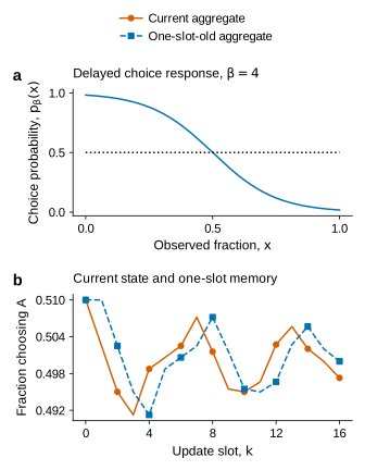
One apparently small indexing choice changes the mathematics. The history stored for the next slot must be the aggregate before the current group updates. Storing the new aggregate instead would remove the intended information delay. A simulation could then look more stable simply because it had quietly been given fresher information.
For this reason, the state immediately before a slot contains five quantities: four group fractions and the previous aggregate. The current aggregate can be calculated from the four fractions, but the previous one must be remembered. All components remain between zero and one under the response rule, provided the initial fractions and history are admissible.
A slot is an opportunity for one whole group to reconsider. It is not a minute, a customer served or a journey completed. Comparisons below keep this unit fixed. Giving one policy additional updates per slot would answer a different question, just as secretly reducing its delay would.
The model also deliberately excludes several real-world features. Options have equal capacity; group sizes and response strengths are initially identical; choices do not change service speeds; and the schedule is specified in advance. These simplifications create a clean test of timing. They do not establish that the same parameter values describe any particular community.
Equal frequency is not equal spacing
There are several different statements hidden inside the word “fair.” A schedule can give all groups the same long-run frequency while permitting very long intervals for one group. It can prevent long intervals but allocate different total numbers of updates. Even equal opportunities would not establish equal benefits if groups faced different costs.
Here, a balanced periodic schedule means that each group occurs equally often within a repeating period. The hard maximum gap is the largest difference between consecutive update indices for any group, including the jump from the end of one period to the beginning of the next.
Round robin has gaps of four everywhere. The gap-5 schedule alternates gaps of three and five for every group. Its average gap remains four. No extra opportunity has been created, and no group has permanently surrendered its share; what changes is the maximum spacing that the schedule permits.
The boundary between periods must be included. Otherwise, a schedule could place two updates close together near the start of a displayed block and appear fair while hiding a long wait across the block’s end. A periodic schedule is an infinite repeating object, not a page of symbols whose last position is exempt from scrutiny.
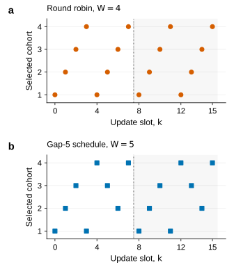
The lower bound is unusually accessible. Suppose . Every consecutive window of four slots must contain every group; if one group were absent, two of its successive updates would be separated by more than four slots. Because there are only four positions, every group appears exactly once.
Now slide that window forward by one position. The group that leaves the window must be the group entering at the other end, or the next window would have a duplicate and a missing group. Therefore . The apparently large family of admissible schedules has collapsed to repeating permutations.
With , even fitting all four groups into every required window is impossible. Thus four is the tightest feasible bound, but feasibility says nothing yet about stability. The question becomes whether the tightest feasible timing pattern is compatible with the dynamics.
This is a useful separation in an optimization problem. First ask which schedules satisfy the opportunity constraint. Then ask what those schedules do to the system. Treating the constraint itself as a performance guarantee skips the second question entirely.
Why order enters the stability calculation
The symmetric state is . To study small disturbances, write deviations from one half as . The response derivative is
The updated group’s first-order deviation is therefore ; the other group deviations are unchanged. The next history deviation is the mean of the old group deviations. Together these relations define a five-by-five update matrix for each selected group.
For a period of length , small deviations at consecutive period boundaries are related by
The earliest update acts first, so its matrix is on the right. Reversing the multiplication order reverses the chronology. The matrices generally do not commute, which is precisely why counting how often each group appears is insufficient.
A useful analogy is applying two different corrections to a document: the second correction acts on the output of the first. Knowing that each correction occurred once does not tell us the final document unless their order is irrelevant. Here, each update changes which group state later contributes to the delayed aggregate.
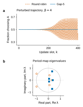
Stability is determined by the eigenvalues of the complete period map. If every eigenvalue has magnitude less than one, sufficiently small disturbances shrink exponentially over repeated periods. An eigenvalue outside the unit circle gives an unstable direction. Eigenvalues on the unit circle require additional analysis; they should not be silently counted as stable.
At , the computed per-slot spectral radii are 1.02867 for round robin and 0.97159 for the displayed gap-5 schedule. These numerical values illustrate the distinction; exact polynomial checks establish the corresponding strict classifications.
The per-slot normalization deserves attention. A longer period gives a system more update opportunities before its period map is measured. Comparing its raw spectral radius with that of a shorter period would mix performance with elapsed time. We instead use
This is an asymptotic local rate, not a promise that every component decreases on every slot. Different modes can interfere, and a stable matrix can show transient amplification. That is why trajectories and initial-state checks remain informative even after the eigenvalues have been certified.
From a convincing plot to an exact statement
A computer can report a spectral radius slightly below one without proving it is below one. Rounding errors matter particularly near a boundary. More importantly, checking several values of does not prove a statement about all values between them.
At the central value , scaled characteristic polynomials of the two period maps are
and
Multiplying a characteristic polynomial by a nonzero constant does not change its roots. These integer forms let the stability calculation avoid floating-point approximations.
The Cayley transformation
turns the unit-disk question into a left-half-plane question. After substituting and clearing the denominator, the scaled polynomials become
and
For a real polynomial with positive leading coefficient, the Routh–Hurwitz criterion tests whether all roots lie strictly in the left half-plane through signs of specific determinants made from its coefficients. For the gap-5 polynomial the five determinants are
All are positive. This proves strict local stability at the central parameter, with no need to round an eigenvalue.
The round-robin polynomial has a different exact argument. Its missing fourth-degree term means the sum of its roots, and therefore the sum of their real parts, is zero. If every real part were nonpositive, all would have to be zero. But an odd-degree real polynomial has a real root; a real root with zero real part would be zero, contradicting the nonzero constant term. At least one root has positive real part.
Transformations have exceptions, so the calculation also checks the excluded points: , , and any loss of degree. Forgetting these checks can turn an elegant argument into an incomplete one.
The proof is stronger than the trajectory picture in one sense and narrower in another. It settles the local classification exactly. It does not identify every attractor far from the equilibrium, prove the eventual oscillations form a particular periodic orbit, or establish chaotic behaviour. A persistent oscillatory trace alone does none of those things.
Certifying a whole interval
The main extension replaces the single central parameter with the closed rational interval . The endpoints were chosen as a tractable sufficient interval around four, not discovered as the exact limits of stability.
For each schedule, we derive the characteristic polynomial symbolically in , form its Cayley polynomial and calculate the Hurwitz determinants. Their coefficients are rational. To prove the required signs throughout an interval, each polynomial is factored and checked using Sturm sequences at the rational endpoints.
The underlying idea is simple even if the intermediate algebra is lengthy. If a continuous polynomial has a known sign at one endpoint and has no root anywhere in the interval, that sign cannot change. Sturm’s theorem supplies an exact count of distinct real roots between endpoints. Endpoint zeros and repeated factors are checked explicitly.
For gap-5, all five Hurwitz determinants and the leading coefficient stay positive. For round robin, the second determinant stays strictly negative. That is not merely a failed strict-stability test: if every root had nonpositive real part, replacing by would move every root strictly left for any positive . Its positive Hurwitz determinants would have nonnegative limits as approached zero. A strictly negative limiting determinant is impossible.
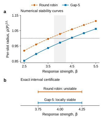
The numerical scan suggests crossings near 3.56033 and 4.43875 for these particular schedules. Those are useful guides, not exact theorem endpoints. A grid can miss a narrow stability island or a tangency; a smooth-looking curve does not prove monotonicity.
Combining the interval certificate with the earlier scheduling argument gives throughout the certified interval. The construction supplies the upper bound. The forced round-robin structure under supplies the lower bound. Neither part can be replaced by a finite search that simply failed to find a better schedule.
The smallest relaxation is not the fastest schedule
The exact minimum-gap result leaves room for a second question: among schedules with an acceptable gap, how fast can small disturbances decay?
We enumerated all 2,520 balanced eight-slot words with two occurrences of each group. At , 1,344 were numerically stable, 408 unstable, and 768 on the numerical boundary. Boundary classifications were retained rather than promoted to success. The best evaluated per-slot radii at exact maximum gaps four, five, six and seven were respectively 1.02867, 0.97159, 0.96388 and 0.89909.
These are statements about that complete finite set. A maximum-gap constraint defines which schedules are allowed, but the actual arrangement still determines the matrix product. Increasing an allowed bound enlarges the design space; it does not make every newly admitted schedule beneficial.
We also examined the 369,600 balanced twelve-slot words with three occurrences of each group, retaining all 1,488 whose cyclic maximum gap was at most five. Of these, 1,176 were numerically stable and 312 unstable; none were classified on the numerical boundary.
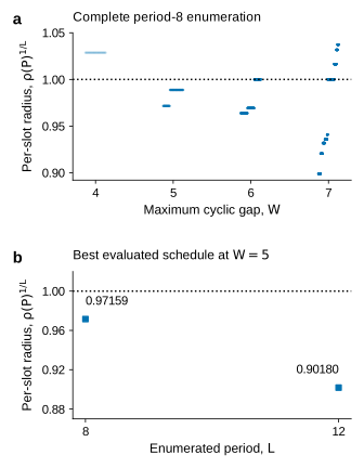
The faster twelve-slot construction is
Its per-slot radius is 0.90180, and its stability at also passes an exact rational certificate. It does not improve the minimum feasible gap, which remains five. Instead, it improves the contraction rate within the searched schedule class.
This is a useful counterexample to stopping at the first successful construction. A proof of existence need not deliver an efficient design. Conversely, an impressive search winner need not be globally optimal. The two claims require different arguments and deserve different wording.
Cyclic rotations and relabeling groups can create equivalent records in these searches. They are retained here to make the candidate counts transparent. Reversing a schedule is not automatically an equivalence: it changes the chronology of the delayed updates and cannot be used as a shortcut without a separate proof.
What happens away from a tiny perturbation?
Local analysis invites a practical challenge: perhaps the stable schedule only helps within an exceptionally small neighbourhood. To investigate without pretending to prove global attraction, we ran deterministic trajectories from seven constant initial fractions: 0.5001, 0.51, 0.49, 0.7, 0.2, 0.95 and 0.05.
We added three nonconstant cases: alternating cohort fractions ; alternating fractions ; and equal current cohort fractions of with a stored previous aggregate of . The first two use stored history . These are specified admissible initial states, not a claim about a preceding equilibrium.
Each case was tested at all four round-robin phases and all eight gap-5 phases, giving 120 main trajectories. Every trajectory ran for 6,000 slots; its final 2,000 slots defined the reported tail statistics. Phase means where the repeating schedule starts, not a new random sample.
For the 40 round-robin cases, tail RMS imbalance ranged from 0.12614 to 0.12622. All 80 gap-5 cases reached a numerically exact equal split in the recorded tail. That zero is a floating-point observation. It does not prove that the mathematical trajectory arrives exactly at equilibrium in finite time.
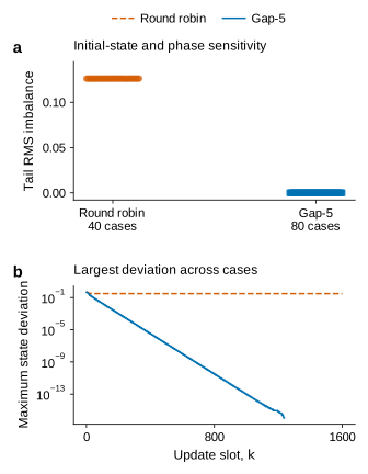
Averaging the two sides’ usage over time would conceal much of this contrast. A system can spend comparable amounts of time above and below one half and have a mean almost exactly equal to one half, while continuing to swing substantially. RMS measures the magnitude of the deviation rather than allowing positive and negative departures to cancel.
The chosen initial states include both small and large disturbances, but they are still a finite collection. They do not cover every possible configuration. A global result would need an additional argument about an invariant attracting region, a suitable Lyapunov function or another mechanism controlling the full nonlinear map.
When groups contain individual agents
A deterministic fraction can be exactly one half. A small group of individuals makes discrete choices and continually introduces sampling fluctuations. Stability of the fraction model therefore does not imply a noiseless finite population.
We simulated 60, 120 and 480 synthetic individuals, divided equally into four fixed groups. When selected, every individual in the group independently chose A with the model probability. Nonselected groups retained their choices. Each run lasted 3,000 slots, with the final 1,000 used for RMS and cost.
Four policies were compared: round robin, the specified gap-5 schedule, independently choosing the next group uniformly at each slot (IID), and reshuffling the order of the four groups at the beginning of each four-slot epoch. There were 20 independent seed-level runs per population and policy, for 240 homogeneous runs.
Within a seed and population, policies shared initial choices and aligned streams of behavioural random numbers. Schedule randomness had a separate stream, so generating a random schedule did not consume the random numbers used for choices. This pairing reduces irrelevant simulation variation, although the policies’ trajectories still diverge after different groups update.
The seeds were already part of development work. Their results remain exploratory; repetition does not turn previously inspected cases into an independent confirmation set. The statistical repetition unit is a complete seed-level run, not an individual slot from its correlated trajectory.
At , mean seed-level RMS values were:
| Policy | Mean RMS imbalance | Hard maximum update gap |
|---|---|---|
| Round robin | 0.13056 | 4 |
| Gap-5 | 0.06772 | 5 |
| IID | 0.05052 | No finite deterministic bound |
| Epoch reshuffling | 0.07103 | 7 |
Gap-5 improves substantially over round robin in this experiment, but it does not have the smallest RMS. IID does. Removing that result would make the story cleaner and less scientifically useful.

The paired gap-5 minus round-robin RMS difference at was −0.06284, with an exploratory 95% bootstrap interval [−0.06570, −0.06014]. The corresponding mean differences were −0.05250 at and −0.08847 at .
A bootstrap interval describes uncertainty in this finite-run comparison under its resampling assumptions. It is not a confidence interval for the exact stability theorem and not a guarantee of performance for an unobserved human population. Both the deterministic proof and the stochastic experiment are valuable, but they answer different questions.
The cost measure is also intentionally transparent:
Its time average equals one half plus twice the squared tail RMS for each run. This identity was checked directly. Reporting lower cost and lower RMS is therefore not two independent pieces of evidence; they are algebraically linked outcomes under an assumed cost function. Neither measures an observed queueing delay.
The benefit of randomness has a price
IID treats groups symmetrically in probability, but it does not guarantee a finite maximum gap. A group can be missed for arbitrarily many consecutive slots with positive probability. Equal expected frequency is not a hard opportunity guarantee.
Epoch reshuffling occupies an intermediate position. Every group appears once in each four-slot epoch, yet one group can be first in one epoch and last in the next. Its consecutive update indices can then be separated by seven slots. Its hard maximum gap is seven, not four.
In the 20 sampled IID schedules of length 3,000, the largest completed observed gaps ranged from 22 to 42 slots. Initial and final incomplete gaps were excluded from this diagnostic. Those finite observations neither establish a hard bound of 42 nor imply that a different run could not contain a longer gap.
The same schedule streams were used at each population size, so repeating that gap range across population settings is expected. It is not several independent discoveries about the gap distribution. Behavioural fluctuations and schedule opportunity patterns have separate sources of variation.
The resulting decision is not “always randomize.” It is to state the acceptable constraint before choosing a performance metric. If no group may wait more than five update indices between opportunities, IID and epoch reshuffling are not comparable feasible substitutes for the certified periodic construction, even if their average imbalance looks attractive.
Where the result stops
We tested two further departures one at a time. First, at , the four groups’ response strengths were multiplied by 0.85, 0.95, 1.05 and 1.15. The same four policies and 20 seeds added 80 synthetic runs. Mean RMS was 0.12767 for round robin, 0.06740 for gap-5, 0.04989 for IID and 0.07252 for reshuffling.
Second, deterministic models with delays zero and two were run from constant initial fraction , using the same 6,000-slot horizon and 2,000-slot tail. Without delay, both periodic policies reached floating-point equilibrium. With delay two, their tail RMS values were 0.24816 and 0.20366, respectively. The gap-5 construction no longer eliminated the sustained imbalance in this test.
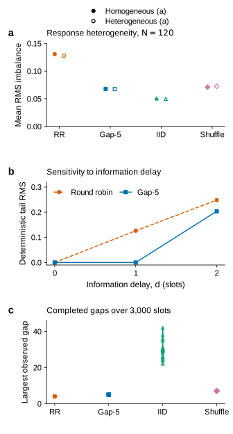
These findings discourage two tempting shortcuts. First, an apparently robust ranking in one heterogeneous setting is not a proof for arbitrary group differences. Unequal responses change the derivative matrices and break the cohort-label symmetry used in the homogeneous lower bound.
Second, a policy that still performs better under a longer delay need not be stable there. Relative improvement and absolute stabilization are separate achievements. A smaller oscillation is not the same as convergence, just as better forecast coverage need not meet a reliability target.
How this connects to earlier research
Timing and delayed interaction have a substantial history. Mosetti, Challet and Solomon studied how desynchronizing minority games changes collective behaviour while preserving their global payoff structure. Their adaptive strategy dynamics differ from the fixed inverse-logistic cohort model here, but the paper is an important warning against treating temporal organization as an irrelevant implementation detail. Structure-preserving desynchronization of minority games.
Colombo and colleagues connect simultaneous stabilization of networked systems to constrained scheduling and maximum disconnection intervals, and develop self-triggered communication rules. That provides a close scheduling perspective. Their separately controlled nodes, Lyapunov conditions and communication design are not the same as our groups coupled through one delayed aggregate. The distinction identifies what must be checked before transferring a theorem; it does not establish that the present construction is new. Simultaneously Stabilizing Networked Systems with Minimal Communication.
Recent work also examines random reshuffling in distributed equilibrium seeking and distinguishes delayed action from delayed information in load balancing. Those mechanisms should not be merged simply because all involve “delay” or “updating.” Here the decision itself uses old information; execution is immediate when a group is selected. Random reshuffling, action-delay load balancing.
The contribution presented in this article is a worked, independently checked model result with an exact parameter-interval extension and bounded computational comparisons. It is not a claim of priority, an accepted paper or a validated intervention.
What should be tested next?
One mathematical direction is to enlarge the certified parameter region. That requires further exact boundary analysis, not merely adding more points to the plotted curve. A different direction is to improve contraction while keeping the gap constraint fixed. The twelve-slot result already shows that period length matters, but it does not settle how much improvement remains available.
A third direction concerns finite populations. The deterministic stability theorem describes a noiseless fraction limit. For a stochastic system with persistent choice noise, an appropriate target might be a bound on stationary imbalance or the probability of a large deviation. Those targets need a stochastic analysis; eigenvalues of an averaged update matrix would not automatically provide it.
Before translating the model into practice, the response law and information structure would also need evidence. Do groups react to current crowding, old reports, expected service time or other people’s choices? Are their memberships fixed? Do updates have unequal costs? A useful model extension should answer one such question explicitly, rather than treating additional complexity as validation by itself.
There is a design lesson even before those extensions. A schedule should be judged on at least three axes: who receives opportunities, how long they can wait between them, and what the resulting feedback does. A policy can improve one axis while worsening another. Declaring a single winner without stating the requirement hides the actual decision.
Conclusion
In this delayed two-choice model, taking turns as evenly as possible is feasible and symmetric, but it is not stabilizing. Allowing the maximum update gap to rise from four to five creates enough scheduling freedom to stabilize the symmetric equilibrium throughout , without increasing anyone’s long-run update share.
The strongest result is the combination of a lower bound and an explicit certified construction. The most useful complications are the faster twelve-slot schedule, IID’s lower simulated imbalance without a hard gap guarantee, and the loss of the original behaviour when the information delay changes.
Fair scheduling is not only about counts. In a feedback system, the order and spacing of opportunities help determine what those opportunities accomplish.
References
- Mosetti, G., Challet, D., and Solomon, S. (2009). Structure-preserving desynchronization of minority games. European Physical Journal B, 71, 573–577.
- Colombo, A., Bahraini, M., Zanon, M., and Falcone, P. (2024). Simultaneously Stabilizing Networked Systems with Minimal Communication. IEEE Transactions on Automatic Control, 69(6), 3589–3601.
- Hu, J., Sun, C., Bo, C., Wang, J., and Wang, Z. (2026). Random Reshuffling-Based Distributed Nash Equilibrium Seeking. Preprint, version 2.
- Abe, K., and Phung-Duc, T. (2026). Load balancing in parallel infinite-server queues with action delay via phase representation. Preprint, version 1.