Assimilating What You Can Observe

A mechanistic model stores states that a surveillance system may never observe. A spatial epidemic model may evolve the susceptible, infected, and recovered populations of every patch, together with parameters and reporting queues. A real report may combine neighbouring regions, arrive late, contain only a fraction of incident cases, and include measurement noise. Passing that report to a filter as though it were the current latent infected state does not merely simplify notation. It changes the statistical problem.

This project turns that distinction into a small, controlled synthetic experiment. One deterministic six-patch SIR trajectory supplies the hidden truth. Four arms share the same truth, 96-member prior ensemble, model, seeds, assimilation dates, and held-out horizon. They differ only in whether and how observations reach the filter: an open loop receives none; an unrealistically direct comparator sees all six latent infected counts; the target arm uses the declared adjacent-pair aggregation, reporting delay, reporting fraction, and noise; and a deliberately misspecified arm applies the wrong grouping, no delay, and the wrong reporting fraction to the same aggregate stream.

The point-estimate result is encouraging. During days 0–44, infected-state RMSE is $264.26$ for open loop, $36.09$ with the correct aggregate-and-delay operator, and $126.34$ with the wrong operator. The correct arm predicts the held-out total-infected peak on the true day, with $0.743\%$ intensity error; the wrong arm is five days late with $4.726\%$ intensity error. Its mean normalized innovation squared is $0.959$ , inside the frozen plausible range.

But the uncertainty result fails. The nominal 90% infected-state interval covers only $0.562963$ of the frozen state-time points, below the predeclared minimum $0.70$ . Four of five recovery gates pass, and the coverage gate does not. The final status is therefore PARTIAL, not fully supported. Good RMSE, plausible average innovation, and an accurate peak do not erase systematic undercoverage.

Everything here is synthetic. “Epidemic,” “reporting,” and “forecast” describe a controlled six-patch mathematical benchmark. No dengue records, patients, districts, case reports, interventions, clinical decisions, or public-health recommendations are involved. The experiment teaches how an observation operator affects state recovery; it does not validate an operational outbreak system.

What the comparison found

Question	Finding	Why it matters
Research context	EnKF epidemic forecasting and observation-function effects are established	This is a focused teaching benchmark, not a new filtering method.
Truth	Deterministic six-patch SIR, 10,000 people per patch	A synthetic latent trajectory, not a fitted disease model.
Prior	Shared 96-member ensemble and fixed seeds	Matched initial uncertainty across all four arms.
Assimilation	Every two days from day 2 through day 44	One frozen update schedule.
Holdout	Day 44 through day 100	No observations are assimilated after day 44.
Correct observations	Three adjacent-pair incidence sums, 0/1/2-day delay weights $(0.15,0.35,0.50)$ , reporting fraction $0.62$	The operator is known by construction, not estimated.
Wrong observations	Non-adjacent pairs, no delay, reporting fraction $0.82$	Deliberate joint misspecification, not an alternative fitted model.
Point recovery	Four of five recovery checks pass	State means and held-out peak forecasts improve under the declared operator.
Uncertainty failure	90% state coverage $0.562963<0.70$	The correct arm is underdispersed on the frozen latent-state comparison.

The comparison prevents several substitutions. The direct latent arm is not the practical winner; it is an optimistic ceiling because it observes what a normal reporting process hides. The correct arm is not “calibrated” merely because its innovation statistic is plausible. A synthetic six-patch result is not dengue evidence merely because dengue motivated the observation-delay question.

Why the literature changed the question

Ensemble data assimilation in epidemic models is well established. Evensen’s sequential ensemble construction laid the EnKF foundation in 1994 (DOI), and Anderson’s ensemble adjustment Kalman filter developed a widely used deterministic alternative and sampling diagnostics (DOI). A local implementation cannot claim to invent ensemble filtering.

In infectious-disease work, Shaman and Karspeck demonstrated ensemble-filter influenza forecasting (DOI). Yamana, Kandula, and Shaman produced dengue outbreak superensemble forecasts (DOI). Pei and colleagues assimilated a spatial metapopulation influenza model (DOI). Liu and colleagues later combined an EnKF with a global spatiotemporal epidemic system (DOI). These works eliminate any novelty claim based on “EnKF plus spatial epidemic forecasting.”

The overlap is closer still. Mitchell and Arnold directly studied observation-function selection in ensemble Kalman filtering for epidemic models, including incidence/prevalence mismatch and under-reporting (DOI). That paper is the decisive reason a broad “observation operators matter” claim is not new. Cocucci and colleagues used ensemble data assimilation when coarse epidemiological aggregates constrain a richer hidden agent state (DOI).

Reporting delay is likewise an established measurement problem. Bastos and colleagues developed a disease-surveillance nowcasting framework with explicit delay correction, including dengue applications (DOI). Yang and colleagues used a delay convolution in Bayesian epidemic assimilation (DOI). Bretó and co-authors formalized plug-and-play inference for partially observed mechanistic systems (DOI), while King and colleagues showed how process and measurement errors can create biased and overconfident outbreak inference (DOI).

Earlier work therefore forces a REFRAME. The defensible contribution is not a new filter, a new dengue model, or a discovery that reporting matters. It is a transparent synthetic stress test that holds truth, prior, dynamics, seeds, and update schedule fixed while contrasting four observation pathways and applying predeclared state, calibration, and held-out peak criteria.

The narrow question is:

In one frozen six-patch synthetic system, how much state and forecast performance does a known aggregate-and-delay observation operator recover relative to open loop and a deliberately wrong operator, and does its uncertainty pass the declared calibration gate?

That last clause is essential. Without it, favorable RMSE could hide an overconfident ensemble.

What the model stores

Each patch $i$ has susceptible, infected, and recovered states. In a generic metapopulation SIR representation,

\frac{dS_i}{dt}=-\lambda_i(t)S_i, \qquad \frac{dI_i}{dt}=\lambda_i(t)S_i-\gamma I_i, \qquad \frac{dR_i}{dt}=\gamma I_i.

The force of infection $\lambda_i$ combines local and neighbouring infected fractions through a frozen ring-mixing matrix. Every patch has population 10,000, local mixing weight $0.76$ , and neighbour weights $0.12$ on either side. Patch-specific transmission coefficients range from $0.22$ to $0.24$ , and recovery rate is $0.105$ . These dimensionless/day-scale parameters create one pedagogical trajectory; they are not estimates for a named pathogen or place.

The truth begins with infected counts $(25,10,3,1,0.5,0.2)$ , while the prior ensemble is centred on $(9,14,6,2,1,0.5)$ . Its transmission-scale multiplier begins with mean $0.78$ rather than the truth value $1$ . The filter therefore has meaningful state and parameter error to correct.

Three incidence queues carry recent simulated incidence so that a 0/1/2-day report can be expressed as a function of model state. This is an important design detail. Delay is not applied as a cosmetic shift to a plotted curve; it is part of the mapping from latent dynamics to observation space.

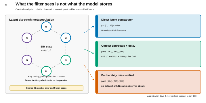
Six-patch latent SIR ring and three observation pathways: unrealistically direct latent counts, correct adjacent-pair aggregation with reporting delay, and deliberately misspecified grouping with no delay. — One truth, model, prior, and seed set; only the observation stream or operator differs. The direct arm is deliberately unrealistic, and the wrong arm consumes the same aggregate stream under false assumptions.

What the filter sees

An observation operator $h$ maps a latent state vector $x$ into the space of measurable quantities:

y_k=h(x_k)+\varepsilon_k, \qquad \varepsilon_k\sim\mathcal N(0,R).

For a linear observation, $h(x)=Hx$ . In this experiment, even the aggregate pathway can be represented through a linear extraction of the augmented state because reporting queues are stored explicitly. The key issue is that $H$ is not the identity matrix.

The direct latent comparator observes all six $I_i$ values with Gaussian standard deviation 18. It asks how the filter behaves when the hidden state is handed over almost directly. That arm is useful for diagnosing the algorithm, but it is not a realistic reporting design.

The correct aggregate-and-delay arm observes three adjacent pair sums: patches $(1+2)$ , $(3+4)$ , and $(5+6)$ . For each pair, reported incidence combines the current and two previous queue entries with weights $(0.15,0.35,0.50)$ and then multiplies by reporting fraction $0.62$ . Gaussian observation standard deviation is 9.

The misspecified arm receives exactly the same noisy aggregate data but interprets them through non-adjacent groups $(1+4)$ , $(2+5)$ , $(3+6)$ , assumes weights $(1,0,0)$ —no delay—and uses reporting fraction $0.82$ . Because grouping, delay, and fraction all change together, the experiment demonstrates joint misspecification damage. It does not identify the isolated causal contribution of each component.

The open loop propagates the same ensemble without analysis updates. It shows how the biased prior evolves in the absence of data.

A compact EnKF update

Let $x_k^{f,(m)}$ be forecast ensemble member $m$ at update time $k$ , with forecast mean $\bar x_k^f$ . Applying the observation operator to every member gives predicted observations $y_k^{f,(m)}=h(x_k^{f,(m)})$ . The ensemble anomalies estimate forecast–observation and observation–observation covariances. A stochastic EnKF update has the form

x_k^{a,(m)} =x_k^{f,(m)} +K_k\left(y_k+\varepsilon_k^{(m)}-y_k^{f,(m)}\right),

where

K_k=P_{xy,k}^f \left(P_{yy,k}^f+R\right)^{-1}.

If $h$ is wrong, the innovation $y_k-y_k^f$ is interpreted in the wrong coordinates. A discrepancy caused by reporting delay may be treated as current-state error. A pair total may push the wrong patches. A reporting-fraction error may be absorbed into the transmission multiplier or infected counts. The Kalman algebra can be internally correct while the measurement semantics are wrong.

After every analysis, this implementation projects epidemiological components to nonnegative values, renormalizes $S+I+R$ to each patch population, and bounds the transmission multiplier in $[0.45,1.55]$ . Those safeguards preserve physical feasibility in the synthetic state. They are algorithmic choices, not proofs of posterior correctness.

A matched four-arm comparison

All arms use assimilation days $2,4,\ldots,44$ and forecast without further observations through day 100. The prior ensemble contains 96 members. Separate frozen seeds control the prior, direct observations, aggregate observations, and each arm’s propagation/update perturbations. No arm is tuned after seeing the final truth.

The main assimilation metrics are infected-state RMSE across all patches and days, mean spatial correlation, empirical 90% interval coverage, interval width, final transmission-scale bias and coverage, and mean normalized innovation squared. The held-out metrics are total-infected RMSE, total interval coverage, peak-day error, and peak-intensity relative error.

The truth’s total-infected peak is $12{,}025.316$ on day 62. Because observations stop on day 44, peak accuracy is genuinely held out from sequential updates, though it remains inside the same synthetic model and parameter family.

Four-panel assimilation-window comparison of patch-one latent infection truth, ensemble mean and 90 percent interval for open loop, direct latent, correct aggregate-delay and misspecified observation operators. — The correct aggregate-and-delay operator markedly reduces point error, but its all-patch empirical 90% state coverage is only 0.563. The figure reports both location and uncertainty rather than hiding the failed gate.

Point recovery: better, but not direct

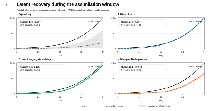
Open-loop assimilation-window infected-state RMSE is $264.255$ , with mean spatial correlation $0.8068$ and coverage $0.3593$ . The biased prior cannot track the growing latent field.

Direct latent observations reduce RMSE to $11.677$ , raise spatial correlation to $0.9601$ , and achieve coverage $0.7481$ . That result establishes an optimistic comparator: its RMSE is $0.3236$ times the correct aggregate arm’s RMSE, below the frozen $0.8$ ratio. The comparison is deliberately unfair in information content and must not be presented as a deployable alternative.

The correct aggregate-and-delay arm achieves RMSE $36.090$ and spatial correlation $0.8523$ . Its RMSE is only $0.1366$ of open loop and $0.2857$ of the wrong-operator RMSE, passing both point-recovery gates by wide margins. The end-of-assimilation transmission multiplier has mean $0.99321$ , bias $-0.00679$ , and a 90% interval $[0.95534,1.02533]$ that contains the truth $1$ .

The wrong operator yields RMSE $126.335$ , spatial correlation $0.8525$ , and transmission-scale bias $-0.03108$ . It recovers some broad spatial co-movement—the correlation is close to the correct arm—while missing amplitude and uncertainty badly. That contrast is a reminder that correlation alone can look favorable when level error remains large.

The correct operator does not recover everything. Aggregating six patches into three pair totals loses within-pair information. Delay mixes recent incidence. Noise and finite ensemble size further limit identification. Even with the observation process known exactly by construction, its state RMSE remains about three times the direct arm’s.

The coverage failure

Nominal coverage is not a decorative uncertainty band. For every fixed patch-day state in the comparison, the experiment checks whether the truth falls between the ensemble’s 5th and 95th percentiles. A well-calibrated nominal 90% interval need not equal exactly 0.9 in one finite dependent sample, but the protocol declares a deliberately broad admissible band $[0.70,0.99]$ . Falling below $0.70$ is treated as material undercoverage; exceeding $0.99$ would flag excessive width.

The correct arm covers only $0.562963$ of state-time points. Its mean interval width is $48.21$ , yet its latent error grows enough that many truth values fall outside. The coverage gate G4 therefore fails.

At the same time, mean normalized innovation squared is $0.9591$ , comfortably inside the frozen $[0.25,2.5]$ interval. These two diagnostics are not contradictory. NIS evaluates innovations in the three-dimensional observed aggregate space using the filter’s predicted observation covariance. State coverage evaluates eighteen-dimensional latent infected values across patches and time. Aggregate innovations can look plausible while conditional uncertainty inside an observed pair is underrepresented.

This distinction is the strongest finding in the benchmark. It shows why observation-space calibration cannot automatically certify latent-state calibration. A filter can explain what it sees and remain too certain about what it cannot separately observe.

Held-out peak forecasts

After day 44, all arms propagate without new observations. Open loop predicts a peak 21 days late and misses intensity by $57.857\%$ ; total-infected holdout RMSE is $5364.98$ . Direct latent assimilation predicts the correct peak day with $0.221\%$ intensity error and holdout RMSE $15.65$ .

The correct aggregate-and-delay arm also predicts the true peak day 62. Its peak-intensity relative error is $0.743\%$ , and holdout RMSE is $59.59$ . The misspecified arm predicts the peak five days late with $4.726\%$ intensity error and holdout RMSE $1493.71$ . Thus the correct operator passes the frozen G6 rule: both its absolute timing and intensity errors are no larger than those from the wrong operator.

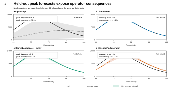
Four held-out total-infected forecast panels from day 44 to day 100, comparing truth with open-loop, direct-latent, correct aggregate-delay and misspecified-operator ensemble forecasts and reporting peak errors. — No observations are assimilated after day 44. The correct operator preserves the true day-62 peak with 0.743% intensity error; the wrong operator is five days late with 4.726% error.

The correct and direct arms both show holdout total 90% coverage of $1.0$ . This does not undo the assimilation state undercoverage. Total infected is a sum across patches and the holdout interval is a different functional over a different time window. Aggregation can cancel patch-level errors, and a total interval can be wide enough to contain the truth even when many individual latent states are missed.

How the comparison was judged

Six declared criteria organize the comparison. G1 is contextual: direct latent RMSE must be at most $0.8$ times correct-operator RMSE for the direct arm to count as an optimistic comparator. It passes at $0.3236$ .

The five core recovery gates are:

G2: correct RMSE / open RMSE $\le 0.85$ . Observed $0.1366$ —pass.
G3: correct RMSE / wrong RMSE $\le 0.8$ . Observed $0.2857$ —pass.
G4: correct state coverage in $[0.70,0.99]$ . Observed $0.562963$ —fail.
G5: correct mean NIS in $[0.25,2.5]$ . Observed $0.9591$ —pass.
G6: correct peak-day and intensity errors no worse than wrong. Observed $0$ days and $0.743\%$ versus $5$ days and $4.726\%$ —pass.

The fixed rule requires all five checks for a fully supported recovery statement. Four pass here, so the point and peak improvements remain valid but the stronger calibrated-recovery statement does not.

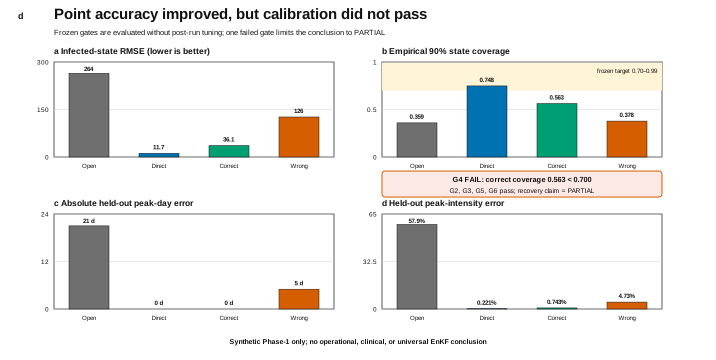
Four-panel results comparison of infected-state RMSE, empirical 90 percent state coverage, held-out peak-day error and peak-intensity error across open, direct, correct and wrong observation arms, with the failed coverage threshold highlighted. — Point accuracy and held-out peak performance improve, but the declared state-coverage target does not pass. That failed uncertainty check prevents a fully supported recovery claim.

This rule blocks a common rhetorical shortcut: reporting only the successful RMSE and forecast panels. The uncertainty failure is co-equal evidence.

Why the metrics disagree

The four principal diagnostics answer different questions and should not be collapsed into one score. RMSE asks whether ensemble means are close to latent truth in the units of infected count. Spatial correlation asks whether the six-patch pattern rises and falls together after removing much of the level and scale information. Empirical coverage asks whether the ensemble’s declared uncertainty contains truth at the promised frequency. NIS asks whether residuals in the three-dimensional observed aggregate space are plausible relative to the predicted observation covariance. A held-out peak functional then asks a fifth question about a derived future total, not about every latent component.

That crosswalk explains several otherwise surprising comparisons. The wrong arm can have correlation $0.8525$ , slightly above the correct arm’s $0.8523$ , while its RMSE is more than three times larger. The correct arm can have NIS $0.9591$ while its latent coverage is only $0.563$ . Correct and direct arms can cover the held-out total at every evaluated time while the correct arm misses many patch-level states during assimilation. None of these results authorizes choosing the most flattering metric; they reveal that each metric projects a different aspect of a partially observed system.

For the same reason, the verdict is not a weighted average designed after seeing the table. The protocol assigns the state-coverage gate a veto over a fully supported recovery claim. If a future study prefers a different hierarchy—for example, prioritising only peak timing—it must declare that estimand and rule before running the experiment. It cannot retroactively rename this benchmark’s failed uncertainty target as irrelevant.

Why the correct arm can still undercover

The observation geometry permits several mechanisms that can produce the observed pattern.

First, aggregation destroys contrast. An adjacent-pair total can be reproduced by many allocations between its two patches. Cross-patch dynamics help reconstruct the split, but they do not create direct measurements.

Second, delay blends time. The observation at one assimilation date contains weighted incidence from the current and previous two queue entries. Even with correct weights, inversion is noisy and correlated across updates.

Third, finite ensembles approximate covariance. Ninety-six members estimate a high-dimensional augmented covariance and can underestimate uncertainty in weakly observed directions. The experiment does not test localization, inflation, larger ensembles, or smoother methods.

Fourth, projection changes distributions. Enforcing nonnegativity, population conservation, and parameter bounds is physically sensible, but nonlinear projection can alter ensemble spread and Gaussian assumptions.

Fifth, model truth equals filter model family. There is no structural process mismatch in the target arm. Real systems would add further uncertainty. If coverage already fails in this favorable closed-world setting, the result argues for caution rather than for extrapolating precise field intervals.

These are plausible explanations, not separately identified causes. The frozen experiment was designed to compare operators, not to attribute undercoverage through an ablation study. A later phase would need to predeclare ensemble-size, inflation, localization, smoothing, and aggregation ablations.

What the wrong arm demonstrates, and what it cannot

The wrong arm jointly changes spatial grouping, delay, and reporting fraction. Its poorer RMSE, forecast, and coverage show that this composite mismatch is consequential in the frozen design. The comparison cannot say whether grouping, delay, or fraction contributes most. It also cannot say that every misspecified operator must perform worse; some wrong models can compensate accidentally under a particular truth.

Its mean NIS is $2.4737$ , just inside the allowed upper boundary $2.5$ , while state coverage is only $0.3778$ . Again, an aggregate observation-space average does not guarantee latent calibration. Its holdout total coverage falls to $0.1754$ , revealing severe forecast underdispersion.

The wrong arm’s spatial correlation $0.8525$ is marginally above the correct arm’s $0.8523$ , despite much worse RMSE and forecasts. That tiny ordering should not be overinterpreted. Correlation removes level and scale information, so an arm can track the general spatial pattern while being badly biased. Multi-metric gates are useful precisely because each statistic has such blind spots.

What this benchmark does not establish

The following claims are outside the evidence:

that a particular dengue surveillance system uses or should use this operator;
that six synthetic patches correspond to districts, hospitals, or communities;
that the declared delay weights or reporting fraction match field data;
that EnKF is superior to particle filters, smoothers, variational methods, or Bayesian alternatives;
that correcting the operator guarantees calibrated latent uncertainty;
that the estimated transmission multiplier is epidemiologically meaningful;
that the held-out peak is an operational forecast;
that an intervention, resource allocation, or health decision should follow from the result;
that the joint misspecification experiment identifies individual causes;
that one deterministic synthetic truth establishes general robustness.

No real person or case record is used. There is no claim of clinical, public-health, or policy readiness.

Why aggregation leaves invisible directions

The simplest pair-total observation already shows the identifiability problem. Ignore delay for a moment and suppose the first report is $y=I_1+I_2$ . The states $(I_1,I_2)=(40,60)$ and $(55,45)$ both produce $y=100$ . Moving along the contrast direction $(1,-1)$ changes the two latent patch values while leaving the observed total unchanged. That direction lies in the null space of the aggregation operator.

With six patches compressed to three adjacent totals, every pair has a similar within-pair contrast. Cross-patch transmission and observations at later dates constrain those contrasts indirectly, but indirect constraint is not direct measurement. If the ensemble covariance becomes too narrow in a weakly observed direction, the three reported totals can remain plausible while individual patch truths fall outside their intervals. That is exactly the pattern behind a reasonable mean NIS and poor latent-state coverage.

Delay adds temporal ambiguity. A high report today can reflect higher incidence today, yesterday, or two days ago because the declared weights mix three queue entries. The dynamics rule out some combinations, but observation noise and two-day update spacing leave others possible. Using the correct operator ensures that the filter asks the right inverse problem. It does not make the inverse problem unique.

This also explains the direct arm. Observing all six $I_i$ values removes much of the spatial null space and avoids the reporting queue, so the arm tests whether the algorithm can track the truth when information is unusually rich. Its lower RMSE is informative about the cost of aggregation. It is not an argument that a surveillance system can collect latent counts that do not exist as direct measurements.

How one wrong update reaches the held-out peak

Consider a report that rises because incidence from the previous two days is now arriving through the delay kernel. The correct arm first generates an equivalent delayed pair total for every ensemble member. Its innovation then measures a difference between predictions and data expressed through the same reporting process. The sample covariance distributes that discrepancy back into patch states, recent incidence queues, and the transmission multiplier.

The wrong arm treats the same number as an undelayed report. It therefore assigns too much of a delayed rise to the current state. It also groups patch 1 with patch 4 rather than patch 2, so the correction can move into the wrong spatial locations. Finally, the assumed reporting fraction $0.82$ interprets a given report as less underlying incidence than the correct fraction $0.62$ would imply. These errors interact, and the filter may partly compensate by changing the transmission multiplier.

Both arms remain nonnegative and conserve population after the update. Their curves can even rise together, which helps explain the wrong arm’s respectable spatial correlation. Numerical feasibility and trend agreement, however, do not make the observation semantics correct. Repeated updates carry the discrepancy into the day-44 ensemble, and that ensemble becomes the initial condition for the observation-free forecast. The five-day peak delay is therefore a downstream consequence of a jointly misspecified update pathway, not evidence that any one of its three errors is solely responsible.

What the numerical verification establishes

Repeating the calculation with the same inputs returned the same state histories, metrics, and coverage failure. Conservation, nonnegativity, observation dimensions, and aggregate-delay calculations also agree with their mathematical definitions. This numerical agreement supports the comparison without extending its empirical scope.

A repeated synthetic result is still synthetic. Matching runs show that the undercoverage is not a one-run accident in this calculation; they do not show that the model is stable across different truths, parameters, networks, or reporting mechanisms. Those questions require a new set of experiments.

What improved, and what did not

The result is not an average of good and bad impressions. The correct operator clearly improves state point estimates relative to open loop and the wrong mapping. It produces plausible mean innovations and a strong held-out peak. Those claims are supported inside the benchmark. The same ensemble does not achieve the declared minimum state coverage, so a broader statement that it recovers the latent field with calibrated uncertainty is not supported.

This wording matters. Saying “the correct operator works” would be too broad. Saying “the correct operator fails” would throw away real point and forecast improvements. The precise claim is:

In this frozen synthetic experiment, explicitly modelling the known aggregation and delay recovers much of the point and peak performance lost to partial observation, but the ensemble remains underdispersed for latent infected states.

That sentence keeps both findings together and makes no operational extrapolation.

What should be tested next

A new protocol could investigate the coverage failure rather than tune it away. Candidate frozen axes include ensemble size, inflation, localization, iterative updates, fixed-lag smoothing, delay-kernel uncertainty, reporting-fraction estimation, pairwise versus larger aggregation, and controlled process mismatch. Each change should be evaluated on multiple held-out synthetic truths rather than one seed family.

An attribution design should vary grouping, delay, and reporting fraction separately and in combinations. That would distinguish which misspecification harms which metric and test whether interactions are additive. A sensitivity panel could also separate observation-space NIS from patch-level state coverage and total-field coverage.

Only after synthetic calibration is understood would real-data work be meaningful. That would require data provenance, reporting definitions, revision and delay processes, privacy governance, a model appropriate to the disease and geography, parameter identifiability analysis, out-of-sample periods, and domain-expert review. Such a study would be a new project, not a footnote to this benchmark.

Conclusion

Data assimilation does not ingest reality. It ingests a measurement model. When a filter’s internal state and a reporting system’s output differ, the observation operator is part of the scientific model, not plumbing around it.

The frozen result makes that point without manufacturing a success. A known aggregate-and-delay operator cuts assimilation RMSE from $264.26$ open loop to $36.09$ , outperforms the wrong operator’s $126.34$ , and preserves an accurate held-out peak. Yet its nominal 90% latent-state interval covers only $56.30\%$ , so the declared full recovery claim fails. The direct latent arm remains an unrealistic upper benchmark, and the wrong arm demonstrates joint misspecification rather than a universal law.

The practical methodological lesson is simple: assimilate what the instrument or reporting process can actually observe, evaluate uncertainty in both observation and latent spaces, and let a failed calibration gate remain visible.