
Twenty-five stable matrices are evidence about twenty-five matrices. A plot of 20,001 stable matrices is much stronger diagnostic evidence, but it is still evidence about a finite set. Neither statement, by itself, proves what happens at every unevaluated parameter value between the plotted points.
A certificate answers a different question. Instead of asking a simulator to visit many parameter values, it asks for one mathematical object whose inequality covers an entire uncertainty set. In this project that object is a positive-definite matrix . If the same satisfies a quadratic Lyapunov inequality at both endpoints of an affine matrix segment, convexity carries the inequality to every matrix between those endpoints. The proof does not depend on whether the interior was sampled 25 times, 20,001 times, or not at all.
That distinction is the subject of P09. The benchmark uses one synthetic two-compartment leaky-transfer family. Its two endpoints are pulled apart through five frozen imbalance levels. At each level, four quantities are placed side by side: a dense spectral sweep, a 25-point seeded spectral sample, a verified quadratic certificate restricted to diagonal , and a verified certificate constructed with a full symmetric .
All six predeclared benchmark checks pass. At zero imbalance, the diagonal and full constructions agree to a relative . At full imbalance, the dense finite diagnostic is , the full certificate is , and the diagonal certificate is . The local diagonal gap relative to the dense diagnostic is . An unchanged repeat returns the same scientific results.
Those numbers support a narrow conclusion: in this fixed two-state family, allowing an off-diagonal term in the constructed quadratic form retains a much less conservative robust decay lower bound at high imbalance. They do not establish a new theorem, a globally optimal semidefinite-program solution, a scaling result, a physical model, a safety guarantee, or a universal superiority law. The study status is PASS (6/6 benchmark checks), and that label goes no further than the six comparisons defined here.
What the certificate establishes
| Question | Result | What it establishes |
|---|---|---|
| State model | Synthetic two-compartment linear system | A transparent mathematical test family, not a calibrated physical process. |
| Uncertainty | One affine line segment at each of five stress levels | Endpoint inequalities can cover every convex mixture in this declared set. |
| Dense diagnostic | 20,001 uniformly spaced values | A fine finite check; explicitly not a certificate. |
| Sparse diagnostic | 25 fixed seeded values | A fixed finite sample; explicitly not a certificate. |
| Certificate construction | Deterministic trace-normalized grid, 241 coarse and 241 refined points per active axis | A search for feasible , not a claim of global SDP optimality. |
| Direct verification | Both endpoint residuals checked after a safety subtraction | The reported positive values are feasible for the complete affine segment. |
| Main contrast at | Dense ; full ; diagonal | A benchmark-specific certificate-quality gap. |
The table prevents several tempting substitutions. A high-resolution curve is not a proof. A feasible matrix from a deterministic search is not a globally optimal SDP solution. A decay bound for a synthetic two-state model is not a physical time constant. Each description stops where its mathematics stops.
Why prior work changed the question
The broad idea is mature. Positive linear systems, Metzler matrices, Lyapunov functions, switching, robust stability, and convex performance analysis have decades of theory behind them. P09 therefore cannot claim that it invented positive-system certificates, diagonal Lyapunov functions, endpoint checking, or scalable convex analysis.
The historical overlap begins well before modern optimization software. Barker, Berman, and Plemmons studied positive diagonal solutions to Lyapunov equations in 1978 (DOI). That work already makes a novelty claim based merely on “positive diagonal Lyapunov matrices” untenable.
The overlap becomes closer for uncertain or switching families. Gurvits, Shorten, and Mason analysed stability of switched positive linear systems (DOI). Mason and Shorten developed linear copositive Lyapunov conditions for switched positive systems (DOI). Knorn, Mason, and Shorten treated common linear copositive Lyapunov functions for sets of positive systems (DOI), while Fornasini and Valcher addressed continuous-time positive switched systems (DOI). These are not distant analogies. They directly occupy the conceptual territory of common certificates across families of positive dynamics.
The literature also extends beyond stability. Tanaka and Langbort gave bounded-real and structured-feedback results for internally positive systems (DOI). Ding, Shu, and Liu further developed copositive Lyapunov conditions for switched positive systems (DOI). Ebihara, Peaucelle, and Arzelier studied -gain analysis for linear positive systems (DOI). Briat treated robust stability, stabilization, and gain characterizations for uncertain positive systems (DOI). A small numerical study cannot plausibly present convex positive-system performance analysis as new.
Later work tightens the boundary still further. Rantzer explicitly developed scalable control formulations for positive systems (DOI); a two-state benchmark has no basis for a new scalability claim. Colombino and Smith gave a convex characterization of robust stability for positive and positively dominated systems (DOI). Gumus and Xu studied common diagonal Lyapunov solutions directly (DOI). Together, these twelve verified primary works make the direct-overlap risk high.
Prior work rules out the original method-novelty headline. The defensible contribution is pedagogical and evidential: build one small family whose complete calculation can be followed, keep finite diagnostics distinct from all-parameter certificates, and measure how a diagonal restriction behaves along a fixed stress path. The local question is:
How does the restriction change a constructed robust decay lower bound as two synthetic leaky-transfer endpoints become more imbalanced, and what exactly is certified by the endpoint inequalities?
That question is useful precisely because it is smaller than the established theory. A reader can follow every matrix, grid choice, residual, and limitation without mistaking the exercise for a new characterization of robust positive systems.
The synthetic leaky-transfer family
Let and consider
The quantities and are positive transfer rates, and are positive removal rates. The off-diagonal entries of are nonnegative, so is a Metzler matrix. For a linear system, that structure preserves the nonnegative orthant: a nonnegative initial state cannot instantly acquire a negative component through the cross-coupling terms.
The column sums are especially transparent:
Transfer moves state between the two coordinates, while the two removal terms leak it from the total. This makes the model structurally interpretable without turning it into a fitted physical system. The words “compartment,” “transfer,” and “removal” name the algebra. They do not identify a biological, chemical, ecological, electrical, epidemiological, or industrial process.
The two frozen full-stress endpoints use the following rates:
| Endpoint | ||||
|---|---|---|---|---|
| Transfer toward compartment 1 dominant | ||||
| Transfer toward compartment 2 dominant |
They generate
Every declared transfer and removal rate is positive. The smallest column leakage anywhere on the five-level path is , above the fixed structural threshold . This is a structural check, not evidence that the numerical rates match any device or population.
Two parameters with different jobs
The experiment uses two scalar parameters, and confusing them would change the design.
First define the midpoint
The stress parameter controls how far the two endpoints sit from that midpoint:
The protocol freezes exactly five values,
At , both endpoints collapse to the same matrix . At , they recover the original imbalanced pair. Thus is a controlled difficulty path, not an uncertain parameter inside one certificate.
At each fixed , the mixture parameter spans the affine uncertainty segment:
The certificate at a particular stress must cover every in that closed interval. The dense and seeded diagnostics evaluate selected values. Keeping and separate makes the scientific question clear: stress changes the family being studied; theta indexes the members that the robust statement must cover.
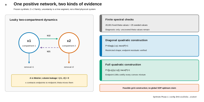
What a spectral simulation does and does not show
For one fixed matrix , define its asymptotic spectral decay diagnostic as
If this number is positive, that fixed matrix is Hurwitz. The dense calculation evaluates this quantity at 20,001 uniformly spaced theta values, so its spacing is . At full stress, the smallest sampled value is
at . The smaller 25-point seeded design finds at . That sparse value is slightly higher because the random design does not land exactly at the narrow minimum seen by the fine uniform grid.
Both calculations are legitimate diagnostics. The dense grid traces the shape of the parameter response and can expose implementation mistakes. The seeded design illustrates what a finite stress test happened to encounter under exact seeds. Neither covers the continuum between its points. Labelling the 20,001-point minimum a “certified worst case” would be a semantic error unless an additional argument bounded the unsampled intervals.
Neither finite diagnostic is a certificate. The dense curve and the 25 seeded points remain sampling comparisons even when their values are close to the constructed lower bound. Tables, plots, and prose must preserve that distinction.
A grid can become part of a valid certification procedure if it is paired with an interval enclosure, a Lipschitz bound, a monotonicity proof, or another mechanism that covers what lies between nodes. P09 does none of those things for the spectral curve. Its robust proof follows a different route: a common Lyapunov inequality.
From a quadratic energy to a decay certificate
Choose a symmetric positive-definite matrix and define
Along ,
Suppose a number satisfies
Then
and therefore
This is the certified statement. It bounds decay in the quadratic energy defined by the constructed . Translating it into a Euclidean norm introduces factors involving the smallest and largest eigenvalues of . P09 does not hide those geometric factors or reinterpret as a measured physical half-life.
For one fixed , the largest admissible alpha for one matrix can be expressed through a generalized eigenvalue calculation. The implementation forms
and takes the smallest generalized eigenvalue of . For a two-endpoint family, the common value is the smaller of the two endpoint values. The runner then subtracts a fixed safety margin and checks the residual matrices directly.
Why two endpoints cover every theta
At fixed stress, assume the same and satisfy
Because , the interior residual is
The cone of negative-semidefinite matrices is convex. Therefore for every . This endpoint implication is standard robust-Lyapunov reasoning; it is not a new theorem contributed by P09.
It also explains why the certificate and the spectral sweep are logically different. The sweep asks for eigenvalues of many individual . The certificate verifies a shared at two endpoint matrices, then uses affinity and convexity to cover the complete segment. More samples may make the first picture smoother. They do not create the second implication.
Diagonal versus full quadratic forms
Scaling by a positive constant does not change feasibility, so the search fixes
Every candidate is parameterized as
For the diagonal construction, and only varies. For the full construction, varies as well, allowing the quadratic energy to tilt relative to the coordinate axes. The coarse search uses 241 points per active axis over its frozen domain, and a second 241-point grid refines the neighbourhood of the best coarse candidate. A 121-plus-121 construction supplies the predeclared resolution sensitivity check.
This parameterization guarantees positive definiteness within the searched interior, but the search remains finite. It constructs a feasible trace-normalized matrix; it does not prove that no other positive-definite matrix yields a larger alpha. An actual global SDP claim would require an appropriate optimization formulation, solver evidence, tolerances, and ideally independent verification. None is asserted here.
The inclusion relation is still informative. The full parameterization contains diagonal candidates at . In a perfectly solved optimization problem, the full optimum could not be worse than the diagonal optimum. In a finite grid search, even that expected ordering must be verified rather than assumed. Repeating the full-stress search with the diagonal candidate included confirms that the reported full value does not underperform it within numerical tolerance.
At , the reported diagonal matrix is
while the full construction is
The off-diagonal term is not a cosmetic embellishment. It rotates the level sets of so that one quadratic form can align better with both imbalanced endpoint dynamics. That geometric explanation is plausible and consistent with the constructed matrices. The numerical result still belongs only to this family; it is not a theorem that every imbalanced positive network needs a full .
Fixing the comparison before evaluation
The two endpoints, five stress values, sample counts, certificate grids, safety margin, normalization, and six acceptance conditions were fixed before the final table was calculated:
- Positive leaky structure: every endpoint must be Metzler and the minimum column leakage must be at least .
- Residual verification: every diagonal and full endpoint certificate must pass the direct matrix check.
- Balanced-limit agreement: at , diagonal and full bounds may differ by at most relative to the dense diagnostic.
- Full-certificate tracking: across the five stresses, the maximum full-to-dense relative gap must be at most .
- Visible diagonal restriction: at , the diagonal relative gap must be at least , while the diagonal certified decay must remain at least .
- Grid sensitivity: changing the construction from 241-plus-241 to 121-plus-121 points may alter no reported bound by more than .
Failure of the first two conditions would invalidate the positive-system or certificate interpretation. Failure of a later condition would preserve any feasible certificate but weaken the comparison attached to it. Results were to be retained in either case.
G3 is a manufactured limiting check, not a discovery. When , the endpoints coincide, so the diagonal and full constructions ought to agree closely in this chosen midpoint case. G5 is deliberately a contrast gate: the family was selected during development to expose a nontrivial restriction gap. Calling it a prediction about naturally occurring networks would reverse the evidence order.
Why the selected family is a teaching example
During preliminary exploration, 240 positive leaky-transfer pairs were screened for valid certificates and a visible diagonal/full contrast. The present family was selected from that pool.
This design step changes the interpretation. The full-stress contrast is not an unbiased estimate of how often diagonal certificates are conservative in a population of systems. The family was intentionally selected because it makes the phenomenon visible while retaining positive leakage and feasible certificates.
The final comparison begins only after the selected family, stress path, grids, thresholds, and success conditions were fixed. A future distributional statement would need a separately defined family-generation mechanism and held-out systems. Reusing the same exploratory pool would not provide such evidence.
Results across the five stress levels
The complete frozen summary is:
| Stress | Dense finite diagnostic | Seeded 25-point diagnostic | Diagonal certificate | Full certificate |
|---|---|---|---|---|
At zero stress, all four quantities nearly coincide because every theta points to the same midpoint matrix. The relative difference between the diagonal and full constructions is , comfortably below the gate.
At , the full and diagonal certificates are still almost indistinguishable from the dense diagnostic. The 25-point minimum is visibly higher because those samples miss the worst region. At , the diagonal restriction begins to lose bound quality: versus a full bound of . At , the diagonal value falls further to , while the full construction remains near .
At full stress, the contrast is largest. Relative to the dense finite minimum, the diagonal gap is
The full gap is only
That closeness is an empirical feature of the frozen family. It does not prove that the full construction found the exact robust decay optimum, nor that a dense spectral minimum is the objective value of a globally solved quadratic-certificate problem. The quantities answer related but distinct questions.
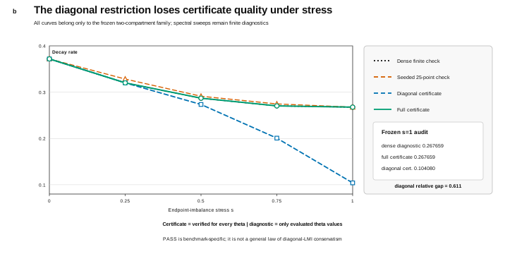
Reading the main figure without overclaiming
Four lines appear on the same axes, but they do not have the same epistemic status.
The dense and seeded curves report minima over evaluated matrices. They are useful for checking shape and for showing how a sparse sample can sit above a narrow adverse region. The diagonal and full curves report positive alphas attached to explicitly stored matrices whose endpoint residuals were verified. Those two curves therefore support all-theta lower-bound statements for their respective quadratic forms.
The diagonal curve falling under stress does not mean the system becomes unstable. Its certified alpha stays positive, including at full stress. The result says the chosen diagonal quadratic form produces a weaker guaranteed rate. A conservative certificate can be small even when every individual matrix appears to decay faster.
Likewise, the full curve tracking the dense diagnostic does not mean the full construction “predicts the truth.” The dense curve is itself finite. The agreement is best read as a consistency observation: a feasible common full quadratic form achieves nearly the smallest spectral decay encountered on the fine grid. It is not a proof that no unsampled matrix has a smaller spectral decay, and it is not a proof that no other improves the certificate.
The stress path also matters. It contracts one selected endpoint pair toward its midpoint. Another path could change leakage, rotate eigendirections differently, alter nonnormality, introduce more vertices, or leave the affine line-segment setting entirely. P09 has not tested those alternatives.
The full-stress theta profile
The full-stress profile makes the evidence hierarchy especially visible. A 401-point curve shows the spectral decay as theta traverses the line segment. The 25 seeded points lie on that curve at their evaluated locations. Horizontal lines show the diagonal and full certificate bounds.
The dense 20,001-point diagnostic places its minimum near , close to the left endpoint but not at it. The smaller seeded set happens to include a point near , so its minimum is close but still optimistic. If the adverse region had been narrower or shifted between random points, the discrepancy could have been larger.
The full horizontal line does not depend on hitting that region. Its logical support comes from the two endpoint residuals. The diagonal horizontal line is supported in exactly the same way, but the restriction on forces it lower for this pair.
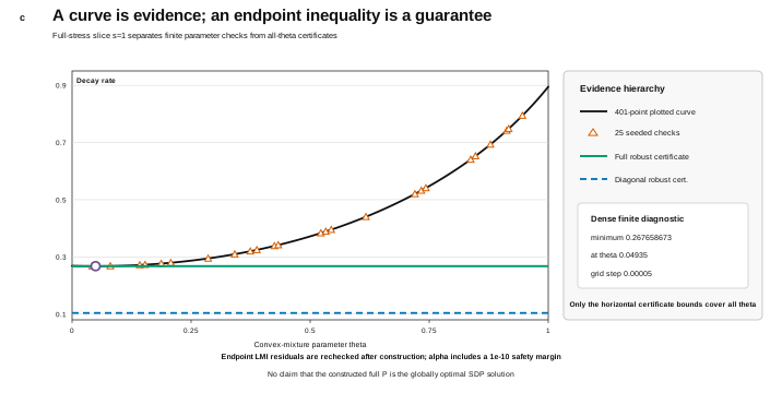
This figure also illustrates why a certificate may lie below a pointwise spectral curve. A single quadratic energy must work for every member of the family. It trades matrix-specific sharpness for a uniform statement. The diagonal restriction removes geometric freedom, so the price of a common form can become larger. None of that implies that quadratic certificates are always necessary, always sufficient for every desired property, or preferable to copositive and positive-system-specific alternatives developed in the literature.
Direct residual checks
After the grid proposes a matrix, the runner recomputes its common generalized decay and subtracts . It then forms, for each endpoint,
and records the largest eigenvalue of the symmetric residual. A nonpositive largest eigenvalue means up to the declared numerical check.
At full stress, the maximum endpoint residual eigenvalue is
for the diagonal construction and
for the full construction. The values are slightly negative, consistent with the deliberate safety subtraction. The stored eigenvalues of both matrices are positive; for the full matrix they are approximately and .
Residual verification is essential because a maximization routine returns only a candidate. A reported alpha becomes a certificate only after the final matrix is shown to be positive definite and the claimed inequality is evaluated directly at the two endpoints.
The residual numbers should still be interpreted with numerical humility. This is binary64 arithmetic with direct eigenvalue calculations, not interval arithmetic or a formally verified proof assistant. The fixed safety margin, hand-checkable cases, and repeated calculation reduce the risk of an inward rounding error, but they do not create machine-checked exact arithmetic.
Grid sensitivity is not an optimality proof
The frozen construction is repeated with 121 coarse and 121 refined points per active axis. The largest absolute change across all diagonal and full values is
below the predeclared threshold. The largest change occurs for the diagonal construction at ; at full stress the diagonal change is about and the full change about .
This comparison is useful because an unstable grid search could produce a visually persuasive but resolution-dependent result. Passing G6 says the reported values do not move much under this one coarsening. It does not prove convergence as grid spacing tends to zero. It does not rule out a better candidate between both grids. And it does not replace an independent conic solver.
For that reason, this article says the search constructs feasible trace-normalized matrices. It does not “solve the SDP.” This may sound like a small wording choice, but it prevents an algorithmic aspiration from being remembered as a verified mathematical outcome.
Structure, feasibility, and the diagonal gap
The first two criteria concern validity. Every endpoint matrix is Metzler, and the minimum leakage is (G1). All 10 constructed certificate matrices satisfy both endpoint inequalities, giving 20 verified inequalities in total (G2). Those facts place the family and the reported certificates inside the declared problem. They do not establish that either grid search found the largest possible alpha.
The next two criteria compare cases where the expected behaviour is known or independently visible. At zero stress, the diagonal and full constructions differ by only (G3). Across the five stress levels, the maximum gap between the full certificate and the dense diagnostic is (G4). The first value confirms the collapsed-family limit; the second shows close agreement on this finite path without turning the dense diagnostic into a proof.
At full stress, the diagonal gap is , while the diagonal certificate remains positive at (G5). The selected family therefore shows substantial but nonzero diagonal conservatism. It does not establish a universal penalty for diagonal Lyapunov matrices. Coarsening the construction from 241 to 121 points changes any reported bound by at most (G6). That is one finite-resolution comparison, not a convergence or optimality proof.
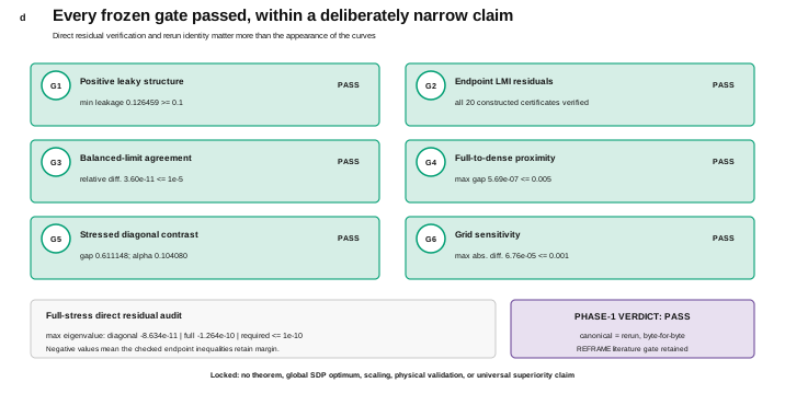
Why the numerical verification is credible
Several independent calculations target different ways the conclusion could fail. Reconstructing the rates checks positivity and leakage; diagonal examples make the spectral abscissa hand-calculable; matrices of the form recover a known generalized decay and reject an invalid alpha; and 101 interior mixtures agree with the endpoint certificate. The full search is also repeated with the diagonal candidate explicitly included, and the complete experiment is repeated while keeping finite diagnostics separate from certificates.
These comparisons do not prove every numerical operation correct. They target errors most likely to change the conclusion: reversing a transfer direction or the Lyapunov inequality, accepting an invalid alpha, omitting the diagonal candidate from the larger family, or relabelling a finite sample as a certificate. The hand-calculable case is especially useful because it supplies an expectation independent of the selected benchmark.
The complete calculation was also repeated independently. The spectral profiles, constructed matrices, residual eigenvalues, and six headline values were unchanged. That agreement supports deterministic execution of this experiment. It does not widen the uncertainty set, strengthen floating-point arithmetic into formal verification, or remove the selection history of the benchmark family.
What this certificate does and does not show
The constructed full matrix is a feasible common quadratic certificate, not a globally optimal one. The diagonal gap belongs to this selected family; it is not a general penalty for diagonal Lyapunov matrices. The dense 20,001-point minimum is still finite, and the 25-point sample is not a probability estimate or confidence interval.
The endpoint argument covers one affine two-vertex segment. It does not cover nonlinear, non-affine, time-varying, or unmodelled uncertainty. The two-state calculation also says nothing about scaling to large sparse networks, computational competition with established methods, or whether a common quadratic form is the best certificate class for positive systems.
The rates do not describe a physical compartment process. The alpha values are not measured decay times, safety margins, reliability levels, or controller guarantees, and no controller was designed. The study supplies neither a new theorem nor a new convex characterization. Its contribution is the transparent comparison between two certificate restrictions and two kinds of finite diagnostic.
Positive leakage also makes broad “discovery of stability” language inappropriate. The family was constructed to be a leaky positive system, and its sampled matrices are comfortably stable. The interesting local quantity is the quality of a robust decay lower bound under a certificate restriction, not a surprise finding that two lossy compartments can decay.
Why finite diagnostics still belong in a certificate study
It would be a mistake to respond to the evidence hierarchy by discarding simulation. The dense curve checks whether the certificate lies in a plausible range, locates the adverse theta region, and exposes the geometry hidden by a single bound. The seeded design demonstrates how finite coverage depends on where points fall. Manufactured cases and interior checks test implementation paths that the endpoint proof alone would not exercise.
The correct relationship is asymmetric. Diagnostics can challenge a certificate implementation: if a sampled matrix decays more slowly than a claimed valid lower bound, something is wrong. But diagnostics do not validate all unsampled matrices merely by becoming dense. A robust workflow uses both, assigns each the right burden of proof, and refuses to let a plot inherit the word “certificate” from the surrounding project title.
That distinction transfers beyond this example. Monte Carlo stress tests, parameter sweeps, scenario libraries, and simulation dashboards answer questions about evaluated cases. A certificate needs a set-wise argument: an invariant, enclosure, convex implication, formal proof, or other mechanism that reaches unevaluated cases. The mechanism may be conservative, but its scope is explicit.
What should be tested next
A more ambitious study would need a new protocol, not a few extra points appended after the result. Useful extensions include larger positive networks, multiple uncertainty vertices, structured parameter blocks, non-affine uncertainty, alternative copositive or diagonal stability conditions, and an independent conic solver with recorded tolerances.
To study general diagonal conservatism, a protocol would need a declared distribution or deterministic library of families, a separation between development and held-out cases, and metrics defined before results are inspected. Candidate selection could then be treated as training, with generalization assessed on untouched networks. Without that separation, more examples selected for dramatic gaps would only reinforce selection bias.
A scaling study would need exact hardware and software environments, sparse versus dense formulations, solver failure accounting, residual checks at comparable tolerances, and sizes large enough to reveal computational structure. P09 contains none of that evidence.
A physical study would require a named system, dimensional units, parameter provenance, uncertainty justification, data or experimental validation, and domain review. A safety claim would require a hazard definition and assurance framework far beyond a quadratic decay bound.
Another useful experiment would rotate the endpoint eigendirections while holding their pointwise spectral decay nearly fixed. That design would isolate the geometric burden placed on a common : a diagonal form cannot rotate with the family, while a full form can tilt its level sets through the off-diagonal entry. Reporting the angle, condition number of , and certificate gap together would make Figure 3’s geometry more explicit without turning one selected stress path into a universal claim.
A second variation would add a third vertex. Endpoint coverage would then mean checking the same inequality at all three vertices, with convexity extending it to the triangle. This would preserve the clean logic of the present certificate while testing whether the diagonal gap is tied to a line segment or persists under a slightly richer uncertainty set. The design should be fixed before selecting a visually dramatic family.
Conclusion
Simulation and certification are complementary, but they are not synonyms. The 25-point and 20,001-point sweeps make the fixed family visible. The endpoint Lyapunov inequalities make an all-theta statement possible. The deterministic grid proposes ; the direct residual check gives each reported alpha its certificate status.
Within this deliberately selected two-compartment family, the diagonal restriction matters. At full imbalance it certifies , while a constructed full quadratic form certifies and the dense finite diagnostic is . That is a clear local contrast, and all six predeclared gates pass.
The durable methodological result is not that full matrices always win. Evidence should be named by the coverage it actually provides. A finite sweep reports what was evaluated. A feasible common inequality covers its declared set. A grid sensitivity check reports one resolution comparison. None should be promoted beyond its own logic.
References
- Barker, Berman, and Plemmons, “Positive Diagonal Solutions to the Lyapunov Equations,” Linear and Multilinear Algebra (1978), DOI 10.1080/03081087808817203.
- Gurvits, Shorten, and Mason, “On the Stability of Switched Positive Linear Systems,” IEEE Transactions on Automatic Control (2007), DOI 10.1109/TAC.2007.899057.
- Mason and Shorten, “On Linear Copositive Lyapunov Functions and the Stability of Switched Positive Linear Systems,” IEEE Transactions on Automatic Control (2007), DOI 10.1109/TAC.2007.900857.
- Knorn, Mason, and Shorten, “On Linear Co-positive Lyapunov Functions for Sets of Linear Positive Systems,” Automatica (2009), DOI 10.1016/j.automatica.2009.04.013.
- Fornasini and Valcher, “Linear Copositive Lyapunov Functions for Continuous-Time Positive Switched Systems,” IEEE Transactions on Automatic Control (2010), DOI 10.1109/TAC.2010.2049918.
- Tanaka and Langbort, “The Bounded Real Lemma for Internally Positive Systems and H-Infinity Structured Static State Feedback,” IEEE Transactions on Automatic Control (2011), DOI 10.1109/TAC.2011.2157394.
- Ding, Shu, and Liu, “On Linear Copositive Lyapunov Functions for Switched Positive Systems,” Journal of the Franklin Institute (2011), DOI 10.1016/j.jfranklin.2011.06.002.
- Ebihara, Peaucelle, and Arzelier, “L1 Gain Analysis of Linear Positive Systems and Its Application,” IEEE CDC/ECC (2011), DOI 10.1109/CDC.2011.6160692.
- Briat, robust stability, stabilization, and gain characterization for uncertain linear positive systems, International Journal of Robust and Nonlinear Control (2013), DOI 10.1002/rnc.2859.
- Rantzer, “Scalable Control of Positive Systems,” European Journal of Control (2015), DOI 10.1016/j.ejcon.2015.04.004.
- Colombino and Smith, “A Convex Characterization of Robust Stability for Positive and Positively Dominated Linear Systems,” IEEE Transactions on Automatic Control (2016), DOI 10.1109/TAC.2015.2480549.
- Gumus and Xu, “On Common Diagonal Lyapunov Solutions,” Linear Algebra and its Applications (2016), DOI 10.1016/j.laa.2016.05.032.