Random Stress Tests Are Not Certificates

A stress test can evaluate thousands of points and still leave the worst point untouched. A local optimizer can land almost exactly on the largest value anyone has seen and still say nothing about values elsewhere in the box. Both tools can produce useful feasible incumbents. Neither one becomes a certificate merely because its best value looks stable.

That distinction is easy to blur in applied work. A table reports the best of 2,048 samples, several seeds agree to four decimals, and a multistart run returns the same candidate from most starting points. The number feels settled. Yet every item in that description is a lower bound on a maximum: each evaluated point proves that the true maximum is at least as large as the best observed value. Certification needs the other side. It needs a valid upper bound on every point that was not evaluated, plus a stopping rule that makes the distance between the feasible lower bound and the set-wise upper bound explicit.

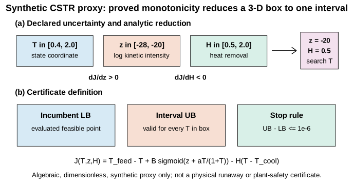
This project builds the smallest example in which that difference can be checked line by line. The objective resembles a thermal-drift score for a continuous stirred-tank reactor, but the resemblance stops at the algebra. It is a synthetic, dimensionless, static function on a bounded box. There is no dynamic reactor state, no heat-capacity model, no physical unit, no calibrated kinetics, no experiment, and no plant-safety boundary. The certificate concerns one mathematical maximum only.

The frozen run succeeds on that narrow task. It returns

1.4443773087849885 \leq \max_{\mathcal U} J \leq 1.4443777214279065,

so the certified gap is

4.1264291805731546\times 10^{-7},

below the declared tolerance of $10^{-6}$ . An independent dense evaluation of 200,001 temperature points gives $1.4443773092028358$ , which lies inside the interval. The dense grid is a useful cross-check, but it does not create the certificate. The upper enclosure does.

The comparison is deliberately uncomfortable. For each fixed IID-uniform and Latin-hypercube budget of 32, 128, 512, and 2,048 points, all 32 seeded replicates miss the declared $10^{-4}$ shortfall rule. That is a record of those exact designs. It is not an estimated miss probability, a confidence statement, or evidence that random sampling usually fails. The local search is stronger in this example: 19 of 32 starts reach within the certificate width. The remaining 13 finish far below. Even the 19 good incumbents have no global upper bound.

What was certified—and what was only sampled

The table separates a mathematical bound from results that come only from evaluated points.

Question	Finding	Why it matters
Research context	Global deterministic bounds, interval methods, sampling designs, scenario theory, and CSTR uncertainty are established	This is a focused benchmark, not a new optimization algorithm or reactor theory.
Uncertainty set	$T\in[0.4,2]$ , $z\in[-28,-20]$ , $H\in[0.5,2]$	One declared rectangular box, not a measured operating envelope.
Reduction	$\partial J/\partial z>0$ , $\partial J/\partial H<0$ on the full box	Every maximizer lies at $z=-20$ , $H=0.5$ .
Certified interval	$[1.4443773087849885,1.4443777214279065]$	The synthetic maximum lies inside this interval.
Gap	$4.1264291805731546\times10^{-7}$	The frozen $10^{-6}$ certificate gate passes.
Dense reference	200,001 temperatures; value $1.4443773092028358$	An independent numerical check lies inside the certificate; it is not the proof.
IID and LHS comparison	$0/32$ hits in each of eight method-budget cells	A design-conditional count for exact seeds, budgets, and the $10^{-4}$ rule.
Multistart local search	19/32 starts within certificate width	Strong feasible incumbents from some starts, no valid global upper bound.

One row deserves emphasis: a dense reference and a certificate answer different questions. The dense grid asks whether a very fine finite set contains a value compatible with the certified interval. It can catch an obvious implementation error. It still leaves gaps between adjacent grid points. The deterministic algorithm must bound those gaps. Calling the grid itself a certificate would silently assume the unsampled variation is harmless.

Why the literature changed the question

The initial project title suggested a new worst-case method for uncertain reactor safety. Current primary literature did not support that headline.

McCormick established convex underestimators for factorable nonconvex programs in 1976 (DOI). Ryoo and Sahinidis developed branch-and-reduce methods with global bounds (DOI), and Sahinidis documented BARON as a general deterministic global-optimization package (DOI). Adjiman, Dallwig, Floudas, and Neumaier gave the theoretical basis for alphaBB on smooth nonconvex problems (DOI). More recent work by Deussen and Naumann uses monotonicity and separability inside interval branch-and-bound (DOI), close in spirit to the coordinate reduction used here. Moeller and colleagues compare a rigorous interval maximization with stochastic and local methods in a different application (DOI).

Sampling has its own mature literature. McKay, Beckman, and Conover introduced the Latin-hypercube design comparison in 1979 (DOI). Scenario results by Calafiore and Campi (DOI) and Campi and Garatti (DOI) do offer probability statements, but under declared random, convex, and support assumptions. A finite stress-test table cannot borrow those guarantees without satisfying their hypotheses.

The reactor context is also established and materially richer than this proxy. Uppal, Ray, and Poore studied multiplicity and dynamic behavior in non-isothermal CSTRs (DOI). Vajda and Rabitz analyzed parametric sensitivity for a CSTR (DOI). Zaldivar and co-authors developed a general runaway criterion across reactor classes (DOI). Grossmann and colleagues reviewed mathematical programming for process systems under uncertainty (DOI).

The overlap is high. This study therefore claims no new global-optimization algorithm and no new reactor-safety theory. Its purpose is narrower: put a valid upper bound, fixed sampling designs, and multistart incumbents in one experiment, then show which statements follow from each object.

Synthetic three-variable objective, bounded uncertainty box, monotonicity signs, exact corner reduction, and the distinction between a certificate and an incumbent. — The two derivative signs reduce the declared box to a one-temperature problem. The reduction is part of the certificate, not a pattern inferred from samples.

The synthetic objective and its boundary

The function is

J(T,z,H) = T_{\mathrm{feed}}-T +B\,r(T,z) -H(T-T_{\mathrm{cool}}),

with

r(T,z) = \operatorname{sigmoid} \left( z+\frac{aT}{1+T} \right).

The frozen constants are

a=40,\qquad B=3,\qquad T_{\mathrm{feed}}=0.5,\qquad T_{\mathrm{cool}}=0.2.

The uncertainty set is

\mathcal U = [0.4,2]\times[-28,-20]\times[0.5,2],

with coordinates $(T,z,H)$ . The notation hints at temperature, a logarithmic kinetic factor, and heat removal. It does not attach physical units or identify a reactor. The score $J$ is an algebraic drift proxy. A positive value is not a runaway declaration. A negative value is not a safe operating certificate.

Why keep the CSTR-like notation at all? It supplies a useful sign structure. The sigmoid reaction term grows with $z$ , while the linear removal term decreases the objective as $H$ grows. Over the frozen temperature interval, $T-T_{\mathrm{cool}}>0$ . Direct differentiation gives

\frac{\partial J}{\partial z} = B\,r(1-r)>0

and

\frac{\partial J}{\partial H} = -(T-T_{\mathrm{cool}})<0.

The derivative check records a minimum $\partial J/\partial z$ of $1.906519333497153\times10^{-7}$ and a maximum $\partial J/\partial H$ of $-0.2$ . The signs therefore hold throughout the full box. Every global maximizer must use the largest allowed $z$ and the smallest allowed $H$ :

z^\star=-20,\qquad H^\star=0.5.

This is an exact reduction. No sample cloud is needed to guess the corner, and no optimizer is trusted to discover it. The three-dimensional problem becomes

\max_{T\in[0.4,2]} f(T), \qquad f(T)=J(T,-20,0.5).

That reduction makes the certificate small enough to inspect, but it also narrows the result. The project certifies a one-dimensional reduced corner problem. It does not certify an arbitrary three-parameter CSTR model, a dynamic trajectory, or a physical uncertainty set.

What the interval algorithm must prove

A global maximization routine needs two quantities.

First, any evaluated feasible temperature $T_k$ supplies a lower bound

L_k=f(T_k)\leq \max_{T\in I} f(T)

for an interval $I$ . The best evaluated value across active intervals becomes the global lower bound, or incumbent.

Second, each interval needs an upper bound $U(I)$ satisfying

f(T)\leq U(I) \quad\text{for every }T\in I.

The requirement covers points that were never evaluated. If an upper formula is merely plausible or empirically tight, the word certificate is not allowed.

The implementation combines two individually valid enclosures and takes their minimum. One uses a nearest-sample Lipschitz argument based on a derivative interval. The other bounds monotone components directly. If the derivative interval has a fixed sign, the proper endpoint is exact for that interval. Otherwise the interval is bisected. A small outward binary64 guard is added so roundoff cannot shrink the claimed upper bound.

The global branch-and-bound state consists of active temperature intervals, their feasible lower values, and their valid upper values. At each step, the interval with the largest upper bound is processed. Its midpoint creates new feasible values and two child enclosures. Intervals that cannot improve the incumbent are harmless, although the tiny frozen run stops before aggressive pruning matters. Termination occurs only when

\max_{I\ \mathrm{active}} U(I)-L_{\mathrm{global}} \leq 10^{-6}.

Notice what is absent. The algorithm does not stop because the best value failed to change for several iterations. It does not stop because 32 starts agreed. It does not stop because a plot looks flat. Those can be practical heuristic criteria, but none supplies the missing upper bound.

How the certified gap closes

The initial interval is wide. Its first recorded upper-minus-lower gap is about $1.61514$ . After one split, the gap is $1.2$ . The reduction then accelerates: by four processed nodes the gap is about $0.07395$ , and by eight nodes it is $2.78556\times10^{-4}$ . Thirteen processed nodes leave five active intervals and close the gap to $4.12643\times10^{-7}$ .

The final feasible lower bound is

L=1.4443773087849885

at the representative point

(T,z,H)=(1.2953125,-20,0.5).

The final upper bound is

U=1.4443777214279065.

An independently constructed 200,001-point temperature grid reports its best value at $T=1.29532$ :

f_{\mathrm{dense}}=1.4443773092028358.

It satisfies $L\leq f_{\mathrm{dense}}\leq U$ . The dense value is slightly above the branch-and-bound incumbent, which is entirely consistent. The certificate never said its representative point was the exact optimizer. It said every possible value lies below $U$ and at least one feasible value reaches $L$ .

Certified lower and upper bounds closing over processed branch-and-bound nodes, with the final gap and certificate interval stated separately. — The deterministic run stops because the valid upper bound minus the feasible lower bound is below $10^{-6}$, not because successive incumbents happen to agree.

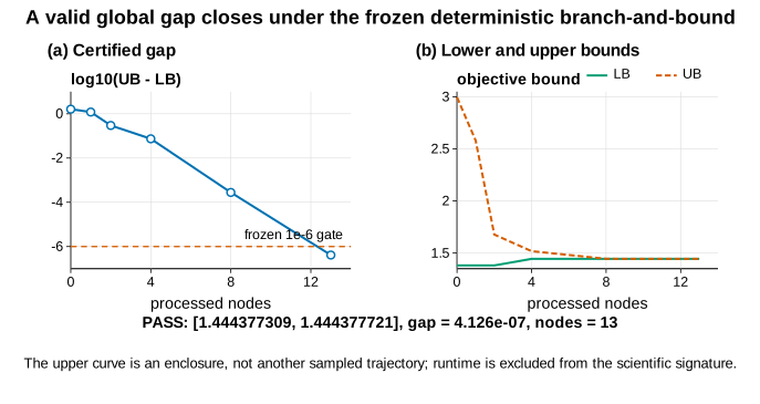
A certificate interval is often more informative than a long decimal printed as “the optimum.” The interval exposes remaining numerical uncertainty. It also forces the implementation to state what has and has not been bounded. Here the uncertainty is algorithmic and set-wise on one synthetic function. It has nothing to do with model-form error, uncertain physical parameters outside the declared box, or plant measurement error.

What the fixed stress tests found

The sampling comparison contains two methods:

IID uniform points drawn independently over the three-dimensional box.
Latin-hypercube points, stratified in each coordinate and randomly paired across coordinates.

Both use budgets 32, 128, 512, and 2,048. Each method-budget cell has 32 fixed replicates with recorded seeds. For a replicate, the best sampled value is a feasible incumbent. A “hit” is declared only if its shortfall from the certified feasible lower bound is at most $10^{-4}$ :

L_{\mathrm{cert}}-\max_{x\in S}J(x)\leq10^{-4}.

Using the certified lower bound rather than the unknown exact maximum makes this a conservative, reproducible reporting rule. It still does not create an upper bound. If a sample hits, one learns that the design found a point close to a known feasible benchmark. If it misses, one learns that this exact finite design did not meet the rule.

All eight cells record zero hits out of 32. Even the largest 2,048-point designs fail the $10^{-4}$ criterion in every fixed replicate. The result is visually striking because the true maximizer sits at two boundary coordinates and a narrow interior temperature. A continuous random design assigns probability zero to landing on the exact $z=-20$ , $H=0.5$ corner. Near-corner points can still score well, but the reaction and removal directions penalize distance from the corner.

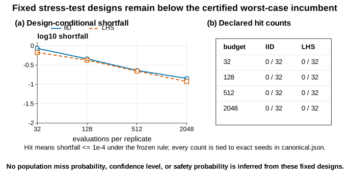
Shortfall distributions for fixed IID-uniform and Latin-hypercube stress tests at four budgets, with every one of 32 replicates missing the declared tolerance. — All displayed zero-hit counts belong to the exact frozen seeds, budgets, uncertainty box, objective, and $10^{-4}$ rule. They do not estimate a general miss probability.

The temptation is to turn “0/32” into “sampling has almost no chance.” The evidence does not permit that sentence. Replicates are fixed computational designs, not a preregistered statistical experiment estimating an unknown Bernoulli parameter. The budgets are four selected values, the dimension is three, and the objective has a particular boundary geometry. No distribution over future problems exists. The project also did not form a binomial confidence interval or verify scenario-optimization assumptions.

A defensible sentence is longer but exact:

None of the 32 frozen replicates for either IID-uniform or Latin-hypercube sampling met the declared $10^{-4}$ shortfall rule at budgets 32, 128, 512, or 2,048.

Every qualifier matters. Remove “frozen” and the seed record disappears. Remove the budgets and the claim sounds asymptotic. Remove the rule and “hit” becomes undefined. Replace “replicates” with “probability” and the claim changes category.

Latin hypercube does improve marginal coverage relative to IID in many integration and design tasks. This experiment is not a verdict against it. Stratifying each coordinate does not guarantee occupation of the particular joint corner that maximizes this function. Another objective, dimension, scrambling, boundary-aware design, or adaptive sampler could behave differently.

Local search gets closer and still lacks a certificate

Projected-gradient multistart uses 32 fixed seeded initial points. Each run stays inside the bounded box and returns a feasible point. Some runs find the reduced worst corner and approach the interior temperature maximum. Others become trapped at poor boundary or stationary configurations.

Nineteen starts finish within the final certificate width of the lower bound. Thirteen remain much farther away. One poor example ends at $T=0.4$ with a value below zero; another reaches only a few millionths above zero. A successful start reaches approximately

(T,z,H)=(1.2953213,-20,0.5)

with value $1.4443773092118821$ , marginally above the branch-and-bound representative incumbent.

This is a good local solution. It is also still an incumbent. The local algorithm did not prove that no better basin exists. Agreement between the good local value and the independent dense reference adds confidence in the implementation, but agreement is not an upper bound.

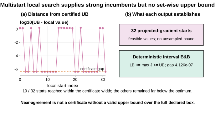
Nineteen of 32 starts reach within the certificate width and 13 remain far below. None of the 32 local runs supplies the certified upper bound.

Names matter here. A local output is a value at a feasible point, together with its shortfall from a known lower benchmark. Calling it a certified optimum would change the mathematical meaning. The plot therefore labels the global upper bound separately from every local value. This avoids a common reporting error: a high feasible result gradually being renamed “worst case” even though no bound was placed over the rest of the set.

The worst-case slice and the exact corner logic

The final diagnostic plots the one-dimensional objective along temperature at the proved corner, together with contrasting slices away from it. The worst-corner curve has an interior peak near $T=1.2953$ . Moving $z$ downward reduces the sigmoid contribution. Moving $H$ upward strengthens removal because $T>0.2$ everywhere in the box. The derivative signs explain the ordering of the slices before any plotting occurs.

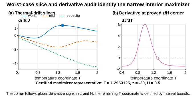
One-dimensional objective slice at the proved worst corner compared with lower slices, with the certified interval and representative temperature marked. — The plot illustrates the reduction already proved by derivative signs. It is not being used to infer monotonicity or certify points between pixels.

The order of evidence matters. First prove the coordinate signs on the full domain. Then reduce the set. Then bound the remaining interval. Finally use the plot to communicate the result. Reversing that order would make a visually plausible pattern carry more authority than it deserves.

The same discipline applies to the independent dense grid. It comes after the valid certificate is defined. Its role is adversarial checking: if the dense value exceeded the upper bound, the enclosure or implementation would be wrong. Because it lies inside, one important inconsistency is absent. But the grid cannot rule out an unseen inter-grid spike by itself.

What validates the certificate

The numerical decision has four clauses:

the monotonicity signs hold on the declared uncertainty set;
the certificate gap is at most $10^{-6}$ ;
the independent dense reference lies inside the interval;
the certificate is accepted only if all preceding clauses pass.

All four pass. No sampling or local-search success is needed for the certificate. Conversely, favorable stress-test results could not rescue an invalid upper bound.

Independent checks exercise derivative signs, interval enclosures, outward guards, branch containment, Latin-hypercube strata, and local projection. An unchanged repeat returned the same certificate interval and gap as well as the same comparator results. These checks support the implementation without expanding what the certificate covers.

The dense grid provides another useful adversarial check. If any of its 200,001 values had exceeded the reported upper endpoint, the certificate implementation would have failed immediately. Its value instead lies within the interval. That agreement does not make the grid a proof, but it removes one clear contradiction between an independently evaluated feasible point and the claimed enclosure.

A repeated calculation cannot broaden the claim. It shows that the reported interval and comparison are not one-run accidents under the fixed inputs. A different box, objective, branch rule, seed schedule, sample budget, or hit tolerance asks a new question and requires a new result.

What every branch preserves

The active branch-and-bound queue represents temperature intervals that have not yet been ruled out. For each interval $I$ , the algorithm stores an upper value $U(I)$ that covers every temperature inside it. Evaluated points supply a global feasible lower bound $L$ . As long as the queue is active, the true maximum must satisfy

L\leq J^*\leq\max_{I\in\mathcal Q}U(I).

This statement is stronger than “the best point has stopped improving.” A stable incumbent describes search history. The inequality still covers the continuum of unevaluated points. Whenever an interval is split, both children need new valid enclosures. A child may be discarded only when its upper bound is no higher than the current incumbent; a poor midpoint is not enough.

Roundoff matters because an upper bound rounded inward can make the final gap look smaller than it is. This experiment uses a conservative outward guard for its fixed, low-dimensional function and checks the bound calculations against dense probes. It does not claim a general directed-rounding system. The logical order remains important: the enclosure must be valid first, then independent evaluations can look for implementation contradictions.

The stopping rule uses the largest upper bound across all active intervals. A narrow interval processed most recently says nothing about another interval whose upper bound remains high. This is why the final $4.1264291805731546\times10^{-7}$ gap compares the incumbent with the most permissive unresolved upper bound, not an average interval width or optimizer step size.

Thirteen processed nodes are enough for this function because two coordinates were removed analytically and the remaining enclosures are tight. That node count is not an efficiency law. A different function, a looser bound, a larger box, or a changed tolerance could require far more work.

What a probability claim would require

Each zero-hit cell answers a narrow design question: for one method, one budget, 32 specified replicates, and the fixed $10^{-4}$ rule, no replicate hit. Turning that count into a miss probability would require an inferential experiment. It would need a defined population of future draws or future optimization problems, a sampling mechanism, an independence model, and a target event chosen before observing the table.

None of those objects is supplied here. The seeds make the computational comparison repeatable; they are not a random sample from a declared population of possible studies. A binomial interval calculated after the fact would therefore attach a probability model that the experiment never specified.

Budget growth also needs careful language. More samples can improve the best feasible value while all runs remain outside a fixed hit tolerance. The best sample still gives a valid lower bound at every budget. It never becomes an upper bound, and relaxing the tolerance after seeing the shortfalls would change the comparison. A future statistical study could estimate design-conditional hit rates, but it would be a separate experiment from this deterministic certificate benchmark.

What the certificate does not say

The largest risk in publishing this example is not numerical. It is linguistic.

The word “CSTR” may invite a reader to imagine a physical reactor. This function has no mass or energy balance in time, no residence-time dynamics, no heat capacity, no coolant dynamics, no feed disturbance, no controller, and no validated constitutive law. Its maximum cannot be translated into a runaway temperature, safe operating limit, alarm threshold, or emergency action.

The word “uncertainty” may invite a probability distribution. The box is a deterministic set. IID and Latin-hypercube points are comparison designs, not a model of how plant parameters vary. No probability measure is attached to $(T,z,H)$ for the certificate. Scenario theory is not invoked.

The word “global” may sound broader than it is. Global means every point in this declared box for this declared algebraic function after a proved coordinate reduction. It does not mean every reactor configuration, every kinetic model, or every source of uncertainty.

The word “certificate” may suggest formal verification of software. The evidence is a mathematically valid numerical bound supported by tests and outward guards. It is not a machine-checked proof in a theorem prover, a regulatory assurance case, or a safety integrity level.

The zero-hit table is also easy to overstate. It cannot support “random stress tests fail,” “Latin hypercube is unreliable,” or “the probability of missing the worst case is near one.” It supports an exact finite statement about 256 design cells in total: two methods, four budgets, and 32 recorded replicates per cell, all evaluated under one hit rule.

Local search receives the same treatment. Nineteen near-certificate starts do not prove that multistart usually succeeds. Thirteen poor starts do not prove that gradient methods usually fail. The only general conceptual statement is definitional: a feasible local incumbent without a valid set-wise upper bound is not a global certificate.

What should be tested next

The present example is intentionally easy enough to verify. Monotonicity removes two coordinates. A next phase should not quietly present the same reduction as a new algorithm. It could test where the clean logic begins to strain:

choose a synthetic objective whose derivative signs change over the box;
compare interval, convex-relaxation, and mixed deterministic bounds under one tolerance;
add dimensions while preserving a provably valid upper enclosure;
predeclare adaptive and boundary-aware sampling designs rather than only IID and LHS;
separate function-evaluation budgets from certification-node budgets;
construct adversarial narrow peaks with known maxima;
use independent implementations of the upper bound;
study directed-rounding or interval-arithmetic libraries explicitly;
if a physical reactor question is intended, start again from a dynamic model, units, data provenance, calibration, validation, and safety-domain review.

Each item changes the research question. None is evidenced by the current run.

A particularly useful comparison would match information fairly. The deterministic method gains exact derivative structure and monotonicity. IID and LHS are deliberately generic. That asymmetry is part of the lesson, but it is not a universal efficiency ranking. A boundary-aware sampler that uses the same derivative signs would immediately concentrate on $z=-20$ , $H=0.5$ . It could find a better incumbent quickly and still lack an upper bound unless it also encloses the remaining temperature interval.

Conclusion

A worst-case report should name both sides of the gap.

A feasible evaluated point gives a lower bound for a maximization. A valid enclosure of every unresolved point gives an upper bound. The difference is the certificate gap. If only the first item exists, report an incumbent, no matter how many samples, starts, or repeated decimals support it.

This project closes that gap to $4.1264291805731546\times10^{-7}$ for one reduced synthetic objective. The result is useful because its boundary is sharp: one box, one function, one tolerance, one analytic corner reduction, and one deterministic interval routine. The fixed random and Latin-hypercube designs happen to record zero hits, while local search often gets very close. Those outcomes make the contrast visible. They do not create probability claims or physical safety evidence.

The final sentence should remain as narrow as the calculation:

For the declared synthetic dimensionless objective on the declared bounded set, the deterministic interval run encloses the global maximum within a gap below $10^{-6}$ ; the fixed seeded sampling and multistart results are feasible incumbents without set-wise upper bounds.

References

Garth P. McCormick, “Computability of Global Solutions to Factorable Nonconvex Programs: Part I, Convex Underestimating Problems,” Mathematical Programming 10 (1976), DOI 10.1007/BF01580665.
Ho-Sung Ryoo and Nikolaos V. Sahinidis, “A Branch-and-Reduce Approach to Global Optimization,” Journal of Global Optimization 8 (1996), DOI 10.1007/BF00138689.
Nikolaos V. Sahinidis, “BARON: A General Purpose Global Optimization Software Package,” Journal of Global Optimization 8 (1996), DOI 10.1007/BF00138693.
Claire S. Adjiman, Stefan Dallwig, Christodoulos A. Floudas, and Arnold Neumaier, “A Global Optimization Method, alphaBB, for General Twice-Differentiable Constrained NLPs, I. Theoretical Advances,” Computers & Chemical Engineering 22 (1998), DOI 10.1016/S0098-1354(98)00027-1.
Jens Deussen and Uwe Naumann, “Subdomain Separability in Global Optimization,” Journal of Global Optimization 86 (2023), DOI 10.1007/s10898-022-01265-6.
Michael Moeller and colleagues, “A Rigorous Deterministic Global Optimization Approach for the Derivation of Secondary Information in Digital Maps,” Optimization and Engineering (2023), DOI 10.1007/s11081-022-09729-0.
Michael D. McKay, Richard J. Beckman, and William J. Conover, “A Comparison of Three Methods for Selecting Values of Input Variables in the Analysis of Output from a Computer Code,” Technometrics 21 (1979), DOI 10.1080/00401706.1979.10489755.
Giuseppe C. Calafiore and Marco C. Campi, “Uncertain Convex Programs: Randomized Solutions and Confidence Levels,” Mathematical Programming 102 (2005), DOI 10.1007/S10107-003-0499-Y.
Marco C. Campi and Simone Garatti, “The Exact Feasibility of Randomized Solutions of Uncertain Convex Programs,” SIAM Journal on Optimization 19 (2008), DOI 10.1137/07069821X.
A. Uppal, W. Harmon Ray, and Aubrey B. Poore, “On the Dynamic Behavior of Continuous Stirred Tank Reactors,” Chemical Engineering Science 29 (1974), DOI 10.1016/0009-2509(74)80089-8.
Sandor Vajda and Herschel Rabitz, “Generalized Parametric Sensitivity: Application to a CSTR,” Chemical Engineering Science 48 (1993), DOI 10.1016/0009-2509(93)81066-5.
Jose M. Zaldivar and colleagues, “A General Criterion to Define Runaway Limits in Chemical Reactors,” Journal of Loss Prevention in the Process Industries (2003), DOI 10.1016/S0950-4230(03)00003-2.
Ignacio E. Grossmann, Robert M. Apap, Bruno A. Calfa, Pablo Garcia-Herreros, and Qi Zhang, “Recent Advances in Mathematical Programming Techniques for the Optimization of Process Systems under Uncertainty,” Computers & Chemical Engineering 91 (2016), DOI 10.1016/j.compchemeng.2016.03.002.