
A numerical method can preserve mass, keep every concentration nonnegative, and approach the correct reduced update as a stiffness parameter vanishes. It can still be less accurate than ordinary backward Euler on every case in a frozen comparison. Those statements do not conflict. They answer different questions.
This distinction matters in fast-slow kinetics because several desirable properties are often compressed into one label. A method is called asymptotic-preserving, robust, physical, or uniformly accurate, and the reader is left to infer that all four descriptions travel together. They do not. Conservation is an algebraic identity. Positivity is a domain property. A fixed-step asymptotic limit concerns what happens when the stiffness parameter tends to zero while the step is held fixed. Accuracy concerns distance from a reference trajectory. Uniform accuracy needs an error statement whose constants do not deteriorate with the small parameter. Runtime superiority requires a controlled cost study. Each claim needs its own evidence.
P08 is a deliberately small study of those separations. It uses one synthetic, dimensionless, irreversible Michaelis-Menten family, one first-order linearly implicit update, ten values of the singular parameter, four fixed step sizes, and one ill-prepared initial condition. It compares the update with a physical backward-Euler solve, classical fixed-step RK4, an exact reduced implicit law, and an internally tightened Radau-IIA-5 reference. The comparison settings were fixed before the final run.
The structural part succeeds. The update conserves the exact weighted invariant by algebra, stays nonnegative with complex concentration at most one, and has the declared fixed-step reduced limit. Tightening the reference changes the trajectory by only , the finest-step error envelope remains below , and the event error remains below . The comparative headline does not survive: at the finest fixed step, the linearly implicit update has higher weighted error than backward Euler for all ten values of the stiffness parameter. The error ratio ranges from 1.0143 to 2.0444.
The useful conclusion is narrower than a new-solver story. On this model, analytic properties and finite-grid accuracy can succeed or fail separately, and a clean property result does not authorize an accuracy or efficiency claim.
What the integrator did across regimes
The main findings fit in one table. Each row answers one numerical question without borrowing support from the rows beside it.
| Question | Measured result | What it means |
|---|---|---|
| Did the tightened reference agree? | Maximum refinement difference | The internal reference is consistent at the scale needed here; it is not an external solver benchmark. |
| Did the linearly implicit update preserve structure? | Invariant drift ; minimum state | The numerical sweep agrees with the algebraic conservation and positivity results on the declared domain. |
| Did it approach the fixed-step reduced update? | Maximum discrepancy | The epsilon sweep supports the stated fixed-step asymptotic limit. |
| Did fixed-step error converge? | Minimum last-pair order | Finite-grid empirical convergence passes; no epsilon-uniform theorem is claimed. |
| Was the finest-step envelope bounded? | Maximum weighted error | The error stays below on the declared grid only. |
| Did it beat backward Euler? | AP/BE error ratio to | No. The comparative hypothesis is null at every tested epsilon. |
| Did fixed RK4 remain physical? | 28 of 40 cases failed or became nonphysical | This is a scoped stiff negative control, not a ranking of adaptive explicit methods. |
| Did the reduced model replace the full state? | Initial complex discrepancy | No. Slow and event agreement improves as epsilon shrinks, but the initial layer remains visible. |
Why prior work changed the question
Michaelis-Menten reduction is not a new setting for singular perturbation analysis. Heineken, Tsuchiya, and Aris treated the quasi-steady-state approximation as a singular limit in 1967. Segel and Slemrod later clarified the fast transient, small parameter, and approximation scales. Modern work by Eilertsen, Schnell, and Walcher maps validity, anti-QSSA regions, initial transients, and error bounds with considerably more care than the familiar textbook derivation.
The numerical side is equally occupied. IMEX and asymptotic-preserving constructions for stiff relaxation have established order conditions and failure modes. Boscarino and Russo studied uniformly accurate IMEX conditions. Schütz and Kaiser developed splitting methods for singularly perturbed ODEs and analyzed order reduction. Most decisively for P08, Kaiser and Schütz published a 2018 analysis of IMEX Runge-Kutta asymptotic error on the Michaelis-Menten singularly perturbed ODE itself, including epsilon sweeps and the differential-algebraic limit. Schütz and Seal later developed a high-order asymptotic-preserving semi-implicit multiderivative method for the broader class.
Positivity and conservation are also established research areas. Sandu studied positive integration for chemical kinetics, while Burchard, Deleersnijder, and Meister gave positive conservative Patankar discretizations for stiff production-destruction systems. Classical IMEX Runge-Kutta, Rosenbrock, VODE/BDF, and Radau methods provide mature comparator families.
The direct overlap is decisive. The literature verdict was REFRAME: P08 cannot claim the first AP or IMEX Michaelis-Menten integrator, a first epsilon sweep, novelty of positivity and conservation, or a new uniformly accurate scheme. The retained question is more modest and more testable:
For one fixed synthetic dimensionless Michaelis-Menten family, can direct analysis distinguish proved conservation, positivity, and a correct fixed-step slow limit from empirical accuracy and stiff-solver performance?
That change gives the computation a clearer job. It checks which properties follow from the formula, which appear only on a finite grid, and whether the proposed accuracy advantage survives a fixed comparison.
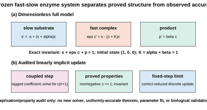
The full model and the initial layer
The dimensionless irreversible Michaelis-Menten system is
with
Here is the substrate-like slow variable, is the fast complex-like variable, and is product. These labels describe the mathematical roles only. No biochemical units, fitted rate constants, measurement errors, or experimental system are attached to them.
Adding the three equations after weighting the complex equation by gives
The initial value is one, so the exact invariant is
The small parameter multiplies the complex derivative. When is small, moves rapidly toward the algebraic slow manifold
Substituting that relation into the slow equation gives the reduced law
The chosen initial condition is ill-prepared because while the algebraic manifold gives
The initial complex discrepancy is therefore exactly for every epsilon. It does not vanish merely because epsilon is small. Instead, it is confined to a progressively shorter fast layer, and its contribution to the weighted invariant is multiplied by epsilon. This is why a reduced model may approximate slow quantities and event times well while failing to reproduce the unweighted fast state near time zero.
That point matters for error definitions. If an error metric gives , , and equal unweighted importance at the initial instant, the reduced model begins with an discrepancy. If the complex component is weighted by epsilon in line with the invariant and singular scaling, its contribution shrinks. Neither metric is universally correct. P08 declares its weighted metric before evaluation and reports the raw complex discrepancy separately so that the weighting cannot hide the initial layer.
A closed-form linearly implicit step
Let . From state and positive step , the linearly implicit update is
The formula is first order and linearly implicit in its derivation, but its implemented step is closed form. There is no Newton iteration and no branch whose convergence depends on an initial guess. That convenience does not make it a new method. Earlier work instead frames it as a simple object whose properties can be tested.
Conservation is an identity
Add the new substrate and product values and then include the weighted complex:
All new-state terms cancel exactly on paper. In binary64 arithmetic the measured maximum drift is . The sweep verifies the implementation, but the finite sweep is not the proof. The proof is the cancellation for every feasible input and positive .
Positivity follows from the same denominator
For nonnegative and positive parameters, is positive and the numerator of is nonnegative, so . The denominator is large enough to bound the new complex by one on the declared feasible set. Rearranging the update with the definition of gives nonnegative forms for and . Product positivity is immediate because it only receives .
Numerical verification extends beyond random states to constructed boundary cases: zero substrate, zero complex, limiting faces of the invariant set, and the full parameter grid. The minimum observed state is exactly zero. Together with the algebra above, this supports the stated property for this update on its feasible input domain; it is not a theorem about arbitrary IMEX schemes or arbitrary reaction networks.
The fixed-step asymptotic limit is explicit
Hold fixed and let . The formula becomes
This is the declared reduced discrete update. The limit is obtained directly from the formula, not inferred from a log-log plot. On the frozen epsilon grid the maximum discrepancy between the full update and this fixed-step limit is , comfortably below the gate.
Calling this property asymptotic-preserving is precise only at the level proved here: for fixed , the scheme has a well-defined epsilon-to-zero update consistent with the chosen reduced discretization. It does not prove uniform accuracy. It does not say that the error constant is independent of epsilon. It does not say the method resolves the fast layer. It does not say that the chosen is appropriate for a biological experiment.
How the reference and comparisons were chosen
The reference is an internal adaptive implementation of three-stage fifth-order Radau IIA. Each implicit stage system is solved with damped Newton iterations. Step doubling controls local error. Reference outputs are generated at all points needed by the fixed-grid comparisons and at extra off-grid times.
The reference calculation needs an independent consistency check. P08 repeats it with tolerances tightened by a factor of ten and compares the trajectories with the same weighted metric used by the study. The maximum refinement difference is , far below the declared tolerance. Reference invariant drift is , and the reference minimum state is zero. Checks away from the final output time reduce the risk that agreement is an artifact of observing only at .
This is strong enough for the Phase-1 comparison, but its scope remains limited. The dependency-free Radau implementation is not a substitute for a work-precision study using mature Radau, BDF, VODE, Rosenbrock, or modern differential-equation libraries. It does not establish speed, robustness across other models, or parity with production software.
The comparison uses
- ten epsilon values from through ;
- four fixed steps ;
- final time ;
- the initial condition ;
- a product event defined by .
The linearly implicit method and backward Euler use exactly the same fixed steps. Backward Euler solves the full nonlinear system through a bracketed physical scalar root, avoiding calibration leakage from the AP formula. Classical RK4 is included as a deliberately simple explicit negative control. The reduced comparator uses the exact scalar implicit Michaelis-Menten update rather than a fitted surrogate.
No tolerance, step, epsilon, metric, or acceptance condition was changed after the output was inspected. A different grid would answer a different question and should be reported as a separate experiment.
What the cross-regime trajectories show
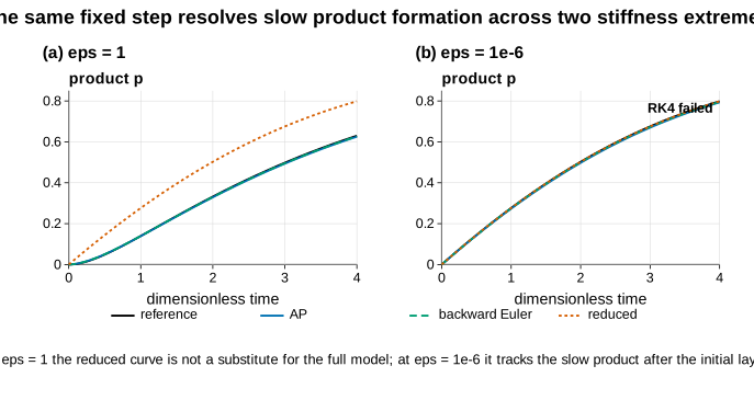
At epsilon one, the complex evolves on a comparable time scale to the slow variables, so replacing it by the algebraic relation is not appropriate. The full reference, linearly implicit update, and backward Euler trace the three-state evolution, while the reduced curve visibly represents a different approximation.
At epsilon , the reference complex moves through a very short initial layer. The slow substrate and product curves quickly align with their reduced counterparts. A fixed output grid can make the fast transient look almost vertical, which is why the property claim is not based on visual smoothness. The full update remains nonnegative and conserves the weighted invariant; those facts come from the formula and its numerical verification.
RK4 supplies a useful contrast. With the same fixed steps it can produce a negative or otherwise nonphysical state when the fast eigenvalue is far outside its stability region. The plot marks that failure instead of clipping the bad trajectory or replacing it with a smaller unregistered step. Yet the result applies only to classical fixed RK4 on this forty-case grid. An adaptive explicit code with stiffness detection is a different algorithm and was not tested.
The two trajectory panels also explain why a single visual verdict would be misleading. At epsilon one, the reduced model removes dynamics that remain visible on the time scale of interest. At epsilon , its slow variables are useful after the initial layer, but the missing half-unit of complex at has not somehow become correct. The approximation improves for selected slow observables because the fast discrepancy is compressed in time and weighted by epsilon, not because every component converges uniformly from the initial instant.
The numerical update has a similar split personality. Its denominator controls positivity and exposes the epsilon-to-zero formula, so those features remain legible even when the trajectory error is not the smallest. Backward Euler, by contrast, pays for a nonlinear solve but obtains lower weighted error on this grid. Figure 2 should therefore be read as a map of regimes and mechanisms. It is not a beauty contest between nearly overlapping curves.
This distinction matters when a model output feeds another calculation. A conserved total may be the right quantity for material accounting. A peak complex concentration may depend on resolving the fast layer. A product threshold may be dominated by the slow accumulation. One integrator can perform differently on all three outputs without contradiction. The correct validation target comes from the quantity eventually reported, not from whichever property is easiest to prove.
The comparison that returned a null result
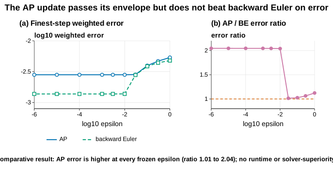
The original comparative hypothesis asked whether the linearly implicit update would have lower weighted error than backward Euler throughout the epsilon grid at the finest fixed step. It does not. For all ten epsilon values,
The minimum ratio is 1.0142693 and the maximum is 2.0444392. In the most favorable case the methods are close, but backward Euler still has the smaller measured error. In the least favorable case the linearly implicit update has roughly double the error.
It would be easy to obscure this result. One could emphasize only the invariant, switch to a component where the curves look closer, choose another step after seeing the table, or present the two methods on a plot whose scale hides the separation. The comparison was fixed in advance, so the null remains: no uniform error advantage over backward Euler appears on the stated grid.
The null does not erase the property result. Backward Euler also has strong stability properties, and on this particular nonlinear system its fully implicit solve is accurate at the selected steps. The linearly implicit update has a simpler closed-form step and a transparent fixed-step limit, but P08 does not measure enough to convert those conveniences into a cost claim. There are no reliable wall-clock comparisons, function-evaluation budgets, linear-solve counts, or production-library baselines.
The conclusion has two parts. The linearly implicit update has the declared structural properties and stays within the finite-grid error envelope. It does not outperform backward Euler in finest-step weighted error on the declared grid. Both clauses must remain together.
Convergence is empirical, not a uniform theorem
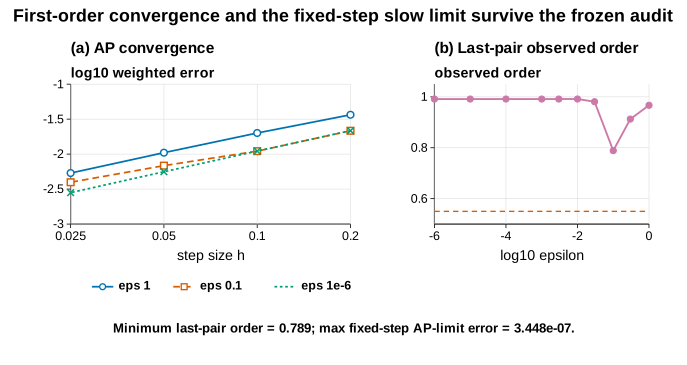
For each epsilon, errors are computed at . The last-pair observed order is
The smallest stored value is , above the preregistered 0.55 floor. First-order behavior is plausible, but four steps and one final time do not prove an asymptotic theorem. Pre-asymptotic effects, reference error, component weighting, and the initial layer can all influence the estimated slope.
The finest-step error envelope takes the maximum weighted error over all ten epsilon values. Its value is , below the frozen 0.025 gate. This is an empirical uniform envelope over a finite list. The adjective uniform here describes the aggregation across the listed epsilon values, not a mathematical bound for every .
The slow-limit panel asks a different question. With fixed, it measures the distance between the full linearly implicit update and the exact limiting discrete update as epsilon decreases. The maximum terminal discrepancy at the smallest registered epsilon is . That diagnostic supports the formula-derived limit and catches implementation errors. It does not measure distance from the continuous reduced solution unless the time discretization error is treated separately.
These distinctions keep three limits from being mixed:
- at fixed epsilon tests time-discretization convergence.
- at fixed tests the discrete asymptotic limit.
- Sending both to zero under a relation between them is a joint-limit question and is not established here.
A uniformly accurate theorem would need bounds with constants controlled independently of epsilon, a precise norm, assumptions on initial preparation, and proof over a continuous parameter interval. P08 supplies none of those ingredients and does not use the phrase as a positive result.
Event timing, feasibility, and the reduced-model boundary
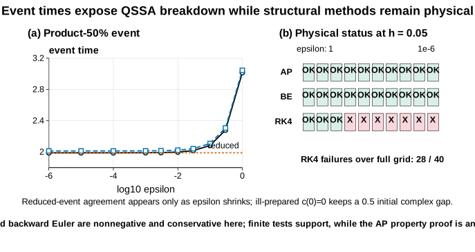
The event is the first time product reaches . Event times are obtained consistently from stored trajectories, with the same interpolation convention for each fixed-step method. The maximum linearly implicit event error at the headline step is , below the fixed 0.08 threshold.
As epsilon shrinks, the reduced model’s product event approaches the full reference event. That agreement is useful because the event depends on the slow accumulation of product. It does not imply full-state agreement at early time. The complex still starts half a unit away from its algebraic value. A paper that reports only event agreement could hide this discrepancy, so Figure 2 and the accompanying discussion retain the ill-prepared initial state explicitly.
The feasibility matrix records whether each fixed method completed without a numerical exception and without violating the declared physical state conditions. Classical fixed-step RK4 fails or becomes nonphysical in 28 of 40 epsilon-step combinations. The failures cluster as stiffness increases and the step becomes too large for the explicit stability region.
This is a negative control with a precise denominator. It is not evidence that explicit integration generally fails for enzyme kinetics. Smaller fixed steps, stabilized explicit methods, adaptive control, exponential integration, or automatic switching can change the result. Nor is the 28/40 count a probability: the forty cells are a deterministic parameter grid, not random draws from a biological population.
Backward Euler remains physical in the comparison because the scalar nonlinear solve is bracketed on the physical interval. That design choice is part of the comparator, not a favor given to the linearly implicit method. The bracket is not tuned with reference answers, and any failed root would remain a failed case rather than being replaced.
How the derivation and numerical results agree
The exact invariant, nonnegative update, bound, fixed-step epsilon limit, physical backward-Euler root, reference refinement, and event interpolation are each checked against the corresponding calculation. A finite collection of numerical cases cannot prove a statement for all admissible states. Its narrower role is to reveal a sign, indexing, root-selection, or interpolation error that would make the computed behaviour disagree with the derivation.
An independent calculation returned the same reference differences, error ratios, event errors, and feasibility pattern. The backward-Euler comparison is therefore not a one-run anomaly under the fixed inputs, although agreement between two calculations does not turn this finite benchmark into a theorem.
The analytic and numerical layers answer different objections. The cancellation proves conservation for the stated feasible set; the calculation confirms that the implemented formula exhibits that cancellation to roundoff. The epsilon limit comes directly from the update; the sweep checks that the computed discrepancy follows it. Reference tightening tests the measuring stick, while backward Euler and RK4 test two different numerical behaviours. Agreement across these layers is stronger than any one plot, yet each layer keeps its original scope.
What this result does and does not show
The system is synthetic and dimensionless. It has no fitted enzyme, substrate, assay, temperature, pH, uncertainty model, or experimental data. The state variables should not be converted into concentrations, doses, clinical endpoints, or process limits.
The update is not presented as a new solver. The direct literature overlap rules out that headline. There is no general theorem of uniform accuracy, no high-order construction, no arbitrary-network result, and no proof for other initial conditions.
The error comparison does not establish backward Euler as universally superior. It concerns one weighted error, one final time, four common fixed steps, and ten epsilon values. Runtime, memory, nonlinear-solve cost, adaptive step selection, tolerance-to-error efficiency, and large-system linear algebra are absent.
The RK4 failures do not rank all explicit methods. The reduced-model agreement does not erase the initial layer. The event result does not validate a biological event. The reference consistency test does not turn an internal Radau implementation into a certified exact solution.
These exclusions are part of the result, not disclaimers added after it.
What should be tested next
A stronger follow-up would start with an externally maintained stiff solver and a published AP or IMEX tableau. It would predeclare tolerance-to-error work-precision metrics, count right-hand-side, Jacobian, factorization, and rejected-step costs, and test well-prepared as well as ill-prepared data. It would include regimes identified by the anti-QSSA literature rather than restricting itself to the present parameter choice.
The work-precision comparison needs special care. Counting steps would favour the closed-form update because a backward-Euler step contains a nonlinear solve. Counting wall time on a three-state Python problem would mostly measure language overhead. A fair study would record residual evaluations, Jacobian work, factorizations, iterations, rejected steps, and memory, then compare errors at matched budgets. Only then could the simple denominator be discussed as an efficiency advantage rather than an algebraic convenience.
Initial preparation should be another experimental axis. With well-prepared data, lies on the slow manifold and the large early discrepancy disappears. With ill-prepared data, the fast layer tests whether accuracy deteriorates when derivatives scale like . Comparing those cases over more parameter regimes would show whether the present error ratios come from the method’s slow dynamics, its treatment of the layer, or both.
For a method contribution, the next phase would need a genuinely new construction or theorem after another novelty review. For an application contribution, it would need physical units, parameter provenance, experimental observations, calibration, validation, and domain review. Those are different projects and should not be merged under one convenient simulation.
P08’s narrower lesson is already useful. A numerical method can have a correct asymptotic limit and exact structural properties without winning an error comparison. A reduced model can predict a slow event while missing the initial fast state. An explicit negative control can fail on most of a frozen grid without supporting a universal claim about explicit algorithms. Keeping those sentences separate produces a more reliable account than selecting a single flattering label.
References
- Heineken, Tsuchiya, and Aris, “On the Mathematical Status of the Pseudo-Steady State Hypothesis of Biochemical Kinetics,” Mathematical Biosciences (1967), DOI 10.1016/0025-5564(67)90029-6.
- Segel and Slemrod, “The Quasi-Steady-State Assumption: A Case Study in Perturbation,” SIAM Review (1989), DOI 10.1137/1031091.
- Eilertsen and Schnell, “The Quasi-Steady-State Approximations Revisited,” Mathematical Biosciences (2020), DOI 10.1016/j.mbs.2020.108339.
- Eilertsen, Schnell, and Walcher, work on anti-QSSA regions, Mathematical Biosciences (2022), DOI 10.1016/j.mbs.2022.108870.
- Eilertsen, Schnell, and Walcher, rigorous initial-transient and approximation-error analysis (2024), DOI 10.1016/j.nonrwa.2024.104088.
- Boscarino and Russo, uniformly accurate IMEX conditions for stiff relaxation, SIAM Journal on Scientific Computing (2009), DOI 10.1137/080713562.
- Schütz and Kaiser, RS-IMEX splitting for singularly perturbed ODEs, Applied Numerical Mathematics (2016), DOI 10.1016/j.apnum.2016.04.004.
- Kaiser and Schütz, IMEX-RK asymptotic error analysis for Michaelis-Menten kinetics, Journal of Computational and Applied Mathematics (2018), DOI 10.1016/j.cam.2018.04.044.
- Schütz and Seal, a high-order AP semi-implicit multiderivative solver, Applied Numerical Mathematics (2021), DOI 10.1016/j.apnum.2020.09.004.
- Sandu, positive numerical integration for chemical kinetic systems, Journal of Computational Physics (2001), DOI 10.1006/jcph.2001.6750.
- Burchard, Deleersnijder, and Meister, positive conservative Patankar discretization, Applied Numerical Mathematics (2003), DOI 10.1016/S0168-9274(03)00101-6.
- Ascher, Ruuth, and Spiteri, implicit-explicit Runge-Kutta methods for time-dependent PDEs, Applied Numerical Mathematics (1997), DOI 10.1016/S0168-9274(97)00056-1.
- Rosenbrock, “Some General Implicit Processes for the Numerical Solution of Differential Equations,” The Computer Journal (1963), DOI 10.1093/comjnl/5.4.329.
- Brown, Byrne, and Hindmarsh, “VODE: A Variable-Coefficient ODE Solver,” SIAM Journal on Scientific and Statistical Computing (1989), DOI 10.1137/0910062.
- Hairer and Wanner, “Stiff Differential Equations Solved by Radau Methods,” Journal of Computational and Applied Mathematics (1999), DOI 10.1016/S0377-0427(99)00134-X.
The final claim stays deliberately narrow: for this fixed dimensionless family, the linearly implicit update has proved conservation, positivity, and a correct fixed-step reduced limit, while the finite experiment rejects a uniform error advantage over backward Euler. No biological or solver-superiority conclusion follows.