同一個積分器跨越快慢尺度邊界

一個 numerical integrator 可以精確保存 mass invariant、令所有 concentration 保持 nonnegative，並且在 stiffness parameter 趨近零時落到正確 reduced update；它仍然可以在每一個凍結 comparison case 都比普通 backward Euler 誤差更大。這些結果沒有矛盾，因為它們回答不同問題。

Fast-slow kinetics 很容易把多種性質壓成一個標籤。方法被稱為 asymptotic-preserving、robust、physical 或 uniformly accurate，讀者便可能假設四件事同時成立。實際上，conservation 是代數 identity；positivity 是 state-domain property；fixed-step asymptotic limit 問的是保持 step 不變而令小參數趨零時，離散公式變成甚麼；accuracy 是 numerical trajectory 與 reference 的距離；uniform accuracy 還要有不會隨小參數惡化的 error statement；runtime superiority 則需要受控 cost comparison。每一項都要有獨立證據。

P08 把研究刻意縮至可以逐式檢查的範圍：一個合成、無因次、irreversible Michaelis-Menten family，一個 first-order linearly implicit update，十個 singular parameters、四個 fixed steps 和一個 ill-prepared initial condition。Comparators 包括 physical backward-Euler solve、classical fixed-step RK4、exact reduced implicit law，以及經 tolerance tightening 的 internal Radau-IIA-5 reference。比較設定在 final evaluation 前固定。

結構部分成功。Update 由代數保存 exact weighted invariant、保持 nonnegative 且 complex 不大於一，並有宣告的 fixed-step reduced limit。收緊 reference 後，trajectory difference 只有 $2.5892\times10^{-12}$ ；finest-step error envelope 低於 $0.025$ ，event error 亦低於 $0.08$ 。但最初的 comparison headline 不成立：在最細固定 step，linearly implicit update 對十個 epsilon 的 weighted error 都高於 backward Euler，ratio 介乎 1.0143 至 2.0444。因此結論是：在這個固定比較中，沒有相對 backward Euler 的 uniform error advantage。

因此本文不是「新 solver 全面勝出」的故事，而是一項 property study：analytical properties 與 finite-grid accuracy 可以分開成功或失敗，漂亮的結構證明不能自動授權 accuracy 或 efficiency claim。

積分器跨尺度時有甚麼表現

下表把各個數值問題分開。每一行只回答自己量度的事情，不借用旁邊結果替它增加含義。

問題	量度結果	它代表甚麼
Tightened reference 是否一致？	Maximum refinement difference $2.5892\times10^{-12}$	Internal reference 在本文所需尺度上保持一致；不是 external solver benchmark。
Linearly implicit update 是否保存結構？	Invariant drift $4.2188\times10^{-15}$ ；minimum state $0$	Numerical sweep 與宣告 domain 上的 algebraic conservation 及 positivity 結果一致。
是否趨近 fixed-step reduced update？	Maximum discrepancy $3.4480\times10^{-7}$	Epsilon sweep 支持公式所述 fixed-step asymptotic limit。
Fixed-step error 是否收斂？	Minimum last-pair order $0.7885$	Finite-grid empirical convergence 通過；不是 epsilon-uniform theorem。
Finest-step envelope 是否受控？	Maximum weighted error $0.0053654$	只代表 declared grid 的 error 低於 $0.025$ 。
Error 是否勝過 backward Euler？	AP/BE ratio $1.0143$ 至 $2.0444$	沒有；comparative hypothesis 在全部 tested epsilon 為 null。
Fixed RK4 是否保持 physical？	40 cases 中 28 個 fail 或 nonphysical	只是一個 scoped stiff negative control，不能排名 adaptive explicit methods。
Reduced model 是否取代 full state？	Initial complex discrepancy $0.5$	不能；slow/event agreement 隨 epsilon 變小，但 initial layer 仍存在。

先行研究怎樣改變了問題

Michaelis-Menten reduction 早已是 singular perturbation analysis 的經典例子。Heineken、Tsuchiya 與 Aris 在 1967 年已把 quasi-steady-state approximation 放進 singular limit 架構；Segel 與 Slemrod 後來清楚分析 fast transient、小參數尺度與 approximation error。Eilertsen、Schnell 與 Walcher 的現代研究則仔細整理 validity regimes、anti-QSSA regions、initial transients 和 rigorous error bounds。單憑重新畫一次 QSSA 曲線，不能構成新研究。

Numerical-method 空間同樣已有直接先行工作。Boscarino 與 Russo 研究 stiff relaxation 的 uniformly accurate IMEX conditions。Schütz 與 Kaiser 為 singularly perturbed ODE 建立 splitting methods 並分析 order reduction。對 P08 最關鍵的是 Kaiser 與 Schütz 在 2018 年已直接研究 Michaelis-Menten singularly perturbed ODE 上的 IMEX Runge-Kutta asymptotic error、stage order、epsilon sweep 和 DAE limit。Schütz 與 Seal 後來又提出 high-order asymptotic-preserving semi-implicit multiderivative method。

Positivity 和 conservation 也不是空白領域。Sandu 研究 chemical kinetics 的 positive integration；Burchard、Deleersnijder 與 Meister 建立 stiff production-destruction system 的 positive conservative Patankar discretization。Classical IMEX Runge-Kutta、Rosenbrock、VODE/BDF 與 Radau 都是成熟 comparator families。

所以文獻結論是 REFRAME。P08 不可聲稱第一個 AP/IMEX Michaelis-Menten integrator、第一個 epsilon sweep、positivity/conservation novelty 或新 uniformly accurate scheme。可辯護的 narrow question 是：

對一個固定的 synthetic dimensionless Michaelis-Menten family，direct analysis 能否把 proved conservation、positivity 與 correct fixed-step slow limit，同 empirical accuracy 及 stiff-solver performance 分開？

問題改寫後，計算的任務也更清楚：哪些性質由公式直接推出，哪些只在有限網格上觀察到，而原擬的 accuracy advantage 能否經得起固定比較。

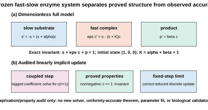
圖卡依次列出無因次快慢酵素模型、exact invariant、linearly implicit update、fixed-step reduced limit，以及比較不涵蓋的新 solver 與 biological claims。 — 模型和 update 足夠小，structure claims 可以直接由公式檢查；圖卡刻意把 algebraic proof 與 finite numerical sweep 分開。

Full model 與 ill-prepared initial layer

Dimensionless irreversible Michaelis-Menten system 是

\begin{aligned} s' &= -s+(s+\alpha)c,\\ \varepsilon c' &= s-(s+\alpha+\beta)c,\\ p' &= \beta c, \end{aligned}

其中

\alpha=0.4,\qquad \beta=0.6,\qquad (s(0),c(0),p(0))=(1,0,0).

$s$ 是 substrate-like slow variable， $c$ 是 fast complex-like variable， $p$ 是 product。這些名稱只描述數學角色，沒有 biochemical units、fitted rate constants、measurement errors 或 experimental system。

把第一與第三條方程相加，再把第二條乘以 $\varepsilon$ ，可得

\frac{d}{dt}\left(s+\varepsilon c+p\right)=0.

初值總量是 1，因此 exact invariant 為

s(t)+\varepsilon c(t)+p(t)=1.

Small parameter 乘在 complex derivative 上。當 $\varepsilon$ 很小， $c$ 快速靠近 algebraic slow manifold

c=\frac{s}{s+\alpha+\beta}.

代回 slow equation 得 reduced law

s'=-\frac{\beta s}{s+\alpha+\beta},\qquad p=1-s.

但 initial condition 是 ill-prepared。因為 $c(0)=0$ ，而 algebraic manifold 在同一 substrate 值給出

c_{\mathrm{qss}}(0)=\frac{1}{1+0.4+0.6}=0.5.

所以 initial complex discrepancy 對每個 epsilon 都是 $0.5$ ，不會因為 epsilon 小便在 $t=0$ 消失。真正發生的是 fast layer 的時間寬度縮短，而 complex 對 weighted invariant 的影響乘上 epsilon。這解釋為何 reduced model 可以逐漸準確預測 slow variables 或 product event，卻不能 uniform 地取代 early-time full state。

Error definition 因而不能含糊。若 $s,p,c$ 在初始時刻用相同 unweighted importance，reduced model 立即有 $O(1)$ error；若 complex component 依 singular scaling 乘上 epsilon，它的 contribution 會縮小。兩種 metric 各自回答不同問題。P08 在 evaluation 前宣告 weighted metric，同時另外公開 raw $0.5$ complex discrepancy，避免 weighting 把 initial layer 隱藏。

這個 model 也說明「physical」在 numerical paper 內很容易被誤讀。本文的 physical state 只代表 nonnegative dimensionless state 並滿足 invariant bounds。它不代表某一種真實 enzyme concentration range，更不表示實驗上可達或生理上安全。

Closed-form linearly implicit step

令 $K=\alpha+\beta$ 。由 state $(s_n,c_n,p_n)$ 和 positive step $h$ 出發，linearly implicit update 是

D=\varepsilon+h(s_n+K+\varepsilon)+h^2\beta,

c_{n+1}=\frac{\varepsilon c_n(1+h)+hs_n}{D},

s_{n+1}=s_n+\varepsilon c_n-(\varepsilon+h\beta)c_{n+1},

p_{n+1}=p_n+h\beta c_{n+1}.

公式在 derivation 上是 first-order linearly implicit，實作時已是 closed form，沒有 Newton iteration，也沒有依賴 initial guess 的 nonlinear branch。這項簡潔性方便檢查，但既有研究不容許把它包裝成 new method。

Conservation 是代數 identity

把新 substrate、weighted complex 與 product 相加：

\begin{aligned} s_{n+1}+\varepsilon c_{n+1}+p_{n+1} &=s_n+\varepsilon c_n-(\varepsilon+h\beta)c_{n+1}\\ &\quad+\varepsilon c_{n+1}+p_n+h\beta c_{n+1}\\ &=s_n+\varepsilon c_n+p_n. \end{aligned}

所有 new-state terms 在紙上 exact cancellation。Binary64 sweep 的 maximum drift 是 $4.2188\times10^{-15}$ 。Finite sweep 用來驗證 implementation，並不是 proof；真正的證明是上述 cancellation 對每個 feasible input 和 positive $h,\varepsilon$ 都成立。

若只從 trajectory 圖看 invariant 幾乎水平，仍不足以知道誤差是否只是 plotting resolution、reference agreement 或 roundoff coincidence。把 algebra 和 finite check 分開，才能清楚指出 claim 的 generality 在哪裏開始和停止。

Positivity 來自同一 denominator

對 nonnegative $s_n,c_n,p_n$ 與 positive parameters， $D>0$ ，而 $c_{n+1}$ numerator 亦 nonnegative，所以 $c_{n+1}\geq0$ 。Denominator 的形式亦足以在宣告 feasible set 上界定 $c_{n+1}\leq1$ 。利用 $D$ 的定義重排，可以把 $s_{n+1}$ 寫成 nonnegative terms； $p_{n+1}$ 更直接，因為它只增加 $h\beta c_{n+1}$ 。

數值核對不只抽一些 random states，亦涵蓋 zero substrate、zero complex、invariant-set faces 與完整 parameter grid 等 boundary cases；觀察到的 minimum state 是 0。連同上面的代數推導，這足以支持該 update 在 feasible domain 內的 property，但不能外推至 arbitrary IMEX scheme、reversible mechanism 或 general reaction network。

Fixed-step asymptotic limit 可直接讀出

保持 $h$ 固定，再令 $\varepsilon\to0$ ，公式變成

c_{n+1}=\frac{s_n}{s_n+K+h\beta},

s_{n+1}=s_n-h\beta c_{n+1},\qquad p_{n+1}=p_n+h\beta c_{n+1}.

這正是 predeclared reduced discrete update。Limit 是從公式得到，不是由 log-log plot 猜測。在 frozen epsilon grid，full update 與 fixed-step limiting update 的 maximum discrepancy 是 $3.4480\times10^{-7}$ ，低於 $2\times10^{-4}$ gate。

因此 asymptotic-preserving 在本文只有一個精確含義：fixed $h$ 下，scheme 有 well-defined epsilon-to-zero limit，而且與所選 reduced discretization 一致。它沒有證明 uniform accuracy、沒有保證 error constant independent of epsilon、沒有 resolve fast layer，也沒有說這個 step 對任何 biochemical experiment 足夠細。

Reference 與 comparators 怎樣選定

Internal reference 使用 adaptive three-stage fifth-order Radau IIA。每個 implicit stage system 以 damped Newton solves 完成，step doubling 控制 local error。Reference outputs 包含 fixed-grid comparison 所需時間點和額外 off-grid points，避免只在 final time 看見偶然一致。

由自己寫的 reference 不能因 method 名字成熟便直接當 truth。P08 以十倍 tighter tolerances 重算，並用同一 weighted metric 比較 trajectories。Maximum refinement difference 是

2.5892155086637556\times10^{-12},

遠低於預先指定的 $5\times10^{-8}$ tolerance。Reference invariant drift 為 $2.4424906541753444\times10^{-15}$ ，minimum state 為 0。這些核對足以支持本文 comparisons，但不等於 external software validation。

Dependency-free Radau implementation 不能取代成熟 Radau、BDF、VODE、Rosenbrock 或 modern differential-equation libraries 的 work-precision study。本文沒有比較 tolerance-to-error curve、rejected steps、Jacobian evaluations、factorizations 或 large-system cost。它只把 internal reference 收緊至 frozen comparison 所需的可信度。

固定的 parameter grid 包含十個 epsilon，由 $1$ 至 $10^{-6}$ ；四個 steps $0.2,0.1,0.05,0.025$ ；final time $4$ ；initial state $(1,0,0)$ ；以及 $p=0.5$ 的 product event。Linearly implicit method 與 backward Euler 共用相同 fixed steps。Backward Euler 以 bracketed physical scalar root 解 full nonlinear system，沒有從 AP formula 偷取 calibration。Classical RK4 是簡單 explicit negative control，reduced comparator 則使用 exact scalar implicit Michaelis-Menten law。

任何 tolerance、step、epsilon、metric 或 acceptance condition 都沒有在看到 output 後修改。若另選 initial condition 或較有利 component，便是另一個實驗，不能覆蓋現在的 null result。

跨越 nonstiff 與 stiff regime

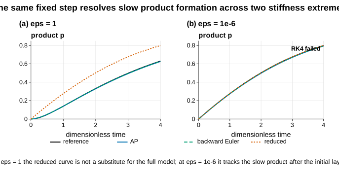
兩個 trajectory panels 比較 reference、linearly implicit method、backward Euler、reduced dynamics 與 fixed RK4，涵蓋 nonstiff 至 epsilon 等於一百萬分之一的 strongly stiff regime。 — 同一 fixed-step update 由 $\varepsilon=1$ 至 $10^{-6}$ 保持 feasible；small epsilon 時 reduced curve 適合 slow variables，但不會重現 ill-prepared fast state 的 initial discrepancy。

當 epsilon 等於一，complex 與 slow variables 的 time scales 相近，直接以 algebraic relation 取代 complex 並不合理。Full reference、linearly implicit update 與 backward Euler 描述 three-state evolution，reduced curve 則明顯是另一個 approximation。

當 epsilon 為 $10^{-6}$ ，reference complex 經歷極短 initial layer，slow substrate 與 product 很快靠近 reduced counterparts。固定 output grid 可能令 fast transient 看似垂直，所以 property claim 不可由 visual smoothness 推出。Full update 的 non-negativity 與 invariant conservation 仍然來自公式及數值核對。

RK4 提供對照。同樣 fixed steps 在 fast eigenvalue 遠離 explicit stability region 時可以出現 negative 或 otherwise nonphysical state。Figure 原樣標記 failure，沒有裁走壞 trajectory，也沒有事後換小 step。不過這只適用 classical fixed RK4 的 forty-case grid；adaptive explicit code、stiffness detection 或 stabilized explicit method 是另一個 algorithm。

兩個 trajectory panels 還揭示一件容易被曲線外觀掩蓋的事。Epsilon 等於一時，complex 與 substrate 在相近時間尺度上變化，reduced curve 移除了仍然重要的 dynamics。Epsilon 降至 $10^{-6}$ 後，reduced substrate 與 product 在 initial layer 後已很有用，但 $t=0$ 的 complex 仍相差 0.5。Slow variables 變準，是因為 fast discrepancy 被壓縮到短時間，而且在 invariant 中乘上 epsilon；並不是所有 components 由第一刻起 uniform convergence。

Linearly implicit update 亦有這種分層表現。它的 denominator 令 positivity proof 和 epsilon-to-zero formula 清楚可見，所以即使 trajectory error 不是最小，兩項結構性質仍然成立。Backward Euler 每步需要 nonlinear solve，卻在這組 fixed-step errors 全面較低。Figure 2 應被閱讀為 regime map：它展示哪些 dynamics 在不同 epsilon 下主導，而不是要求讀者憑幾條接近的 curves 選出「最好」方法。

最後使用哪一個輸出，會改變最需要驗證的誤差。若目標是 material accounting，weighted conserved total 最重要；若目標是 peak complex，initial layer 不可被 reduced model 省略；若目標是 product crossing，slow accumulation 和 interpolation 會主導 event time。一個 integrator 在三種輸出上可以有三種相對表現，並不矛盾。Validation 應從最後要報告的 quantity 反推，而不是由最容易證明的 property 代替全部問題。

必須保留的 comparative null

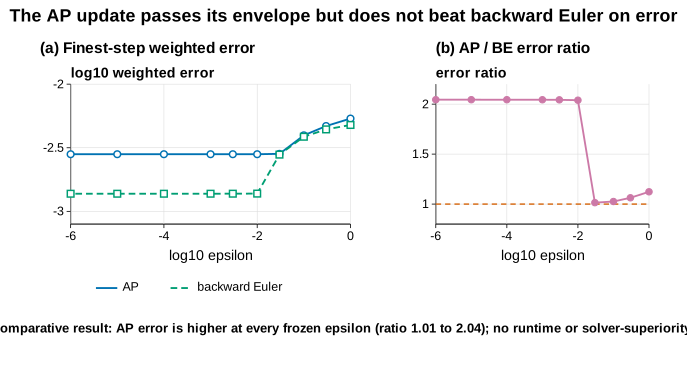
十個 epsilon 上 linearly implicit AP update 與 backward Euler 的 finest-step weighted errors，以及全部高於一的 AP-to-BE error ratio。 — 固定 $h=0.025$ grid 上每一個 ratio 都大於一；structure checks 通過，但 proposed uniform error advantage 被拒絕。

Original comparative hypothesis 問：在 finest fixed step，linearly implicit update 是否於整個 epsilon grid 都比 backward Euler 有較低 weighted error？答案是沒有。十個 epsilon 全部滿足

\frac{E_{\mathrm{AP}}}{E_{\mathrm{BE}}}>1.

Minimum ratio 是 1.0142693，maximum 是 2.0444392。最接近的一個 case 兩者差很少，但 backward Euler 仍然較低；最不利 case 則 linearly implicit update 約有兩倍 error。

這個結果很容易在寫作時被淡化。可以只談 invariant、改用另一個 component、看完 table 再選 step，或者用太寬 y-axis 把差異壓平。比較方式已經固定，所以不能把這個 null 改寫成 accuracy advantage。

Null 不會抹去 property result。Backward Euler 本身是成熟 stiff method，在這個 nonlinear system 的 selected steps 亦可以很準確。Linearly implicit update 有 closed-form step 和透明 fixed-step limit，但 P08 沒有足夠 evidence 把這些便利轉成 cost superiority。沒有可靠 wall-clock comparison、function-evaluation budget、linear-solve count 或 production-library baseline。

結論必須包含兩句：linearly implicit update 有已證的 structural properties，並保持在 finite-grid error envelope 內；它在 declared grid 的 finest-step weighted error 沒有勝過 backward Euler。只保留第一句會扭曲實驗目的，只保留第二句又會忽略真正已證的 algebraic properties。

Convergence plot 不是 uniform theorem

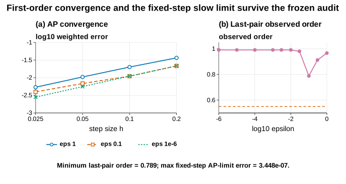
Selected epsilon values 的 fixed-step log-log convergence curves，旁邊是 full update 與 reduced fixed-step limit 的 discrepancy。 — Observed last-pair orders 與 slow-limit discrepancy 通過 frozen gates；它們是 finite-grid diagnostics，不是 epsilon-uniform convergence proof。

對每個 epsilon，errors 在 $h=0.2,0.1,0.05,0.025$ 計算。Last-pair observed order 定義為

q=\log_2\!\left(\frac{E(h=0.05)}{E(h=0.025)}\right).

最小 stored value 是 $0.7885474783868782$ ，高於 preregistered 0.55 floor。First-order behavior 可信，但四個 steps、一個 final time 不會構成 asymptotic theorem。Pre-asymptotic effects、reference error、component weighting 與 initial layer 都會影響 slope。

Finest-step error envelope 對十個 epsilon 取 maximum weighted error，所得

0.005365433451822332

低於 frozen 0.025 gate。這是有限清單上的 empirical uniform envelope。「Uniform」在這一句只表示 aggregation 跨越列出的 epsilon，並非對所有 $0<\varepsilon\leq1$ 的 mathematical bound。

Slow-limit panel 問另一件事：fixed $h$ 下，full linearly implicit update 和 exact limiting discrete update 的距離如何隨 epsilon 下降。Smallest registered epsilon 的 maximum terminal discrepancy 為 $3.448014616047601\times10^{-7}$ 。這個 diagnostic 支持 formula-derived limit，亦可以捉 implementation error；它沒有直接量度 continuous reduced solution error，除非另外分離 time-discretization error。

三種 limit 不可混為一談： $h\to0$ at fixed epsilon 測試 time convergence； $\varepsilon\to0$ at fixed $h$ 測試 discrete AP limit；兩者按某個 relation 同時趨零則是 joint-limit question，P08 沒有處理。真正 uniformly accurate theorem 還需要 epsilon-independent constants、清楚 norm、initial-preparation assumptions 和 continuous parameter interval。本文沒有提供，故不作正面 claim。

Event timing、feasibility 與 reduced boundary

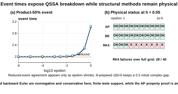
Product-event timing error 隨 epsilon 的變化，旁邊是 method-by-step feasibility matrix，其中 fixed RK4 有 28/40 cases fail 或 nonphysical。 — Headline-step event error 低於 frozen threshold，而 fixed RK4 在 28/40 cases 失敗；兩個數字都只屬於這個 model、grid、event 和 implementation。

Event 定義為 product 首次達到 $p=0.5$ 的時間。各 fixed-step methods 由 stored trajectories 以相同 interpolation convention 找 crossing。Linearly implicit update 的 maximum headline-step event error 是 $0.03040719917476009$ ，低於固定的 0.08 threshold。

Epsilon 下降時，reduced model 的 product event 靠近 full reference event。這項 agreement 有意義，因為 event 依賴 product 的 slow accumulation；但它不表示 early-time full state 相同。Complex 在初始仍然相差 0.5。若文章只報 event accuracy，便會隱藏 initial-layer failure，所以 Figure 2 和正文都保留 ill-prepared discrepancy。

Feasibility matrix 記錄每個 fixed method 是否完成，而且沒有違反 declared physical state conditions。Classical fixed-step RK4 在 40 個 epsilon-step combinations 中有 28 個 fail 或 become nonphysical，主要隨 stiffness 增加、step 超出 explicit stability region 而出現。

28/40 有清楚 denominator，卻不是 probability。Forty cells 是 deterministic grid，不是從 enzyme population 抽出的 random cases。結果不表示 explicit integration 一般有七成 failure rate。Smaller fixed steps、adaptive control、stabilized explicit schemes、exponential methods 或 automatic switching 都可能改變 outcome；本文沒有測試。

Backward Euler 在這項比較保持 physical，因為 scalar nonlinear solve 在 physical interval bracket。這是 comparator design 的一部分，不是只對 linearly implicit method 提供方便。若 root solve failure，該 case 會原樣保留，而不是從 reference 取得初值後重跑。

公式與數值結果如何互相核對

Exact invariant、nonnegative update、 $c\leq1$ bound、fixed-step epsilon limit、physical backward-Euler root、reference refinement 和 event interpolation，都分別對照相應計算。有限數值 cases 不能證明所有 admissible states 的 statement；它們較窄的作用，是揭示 sign、index、root selection 或 interpolation 的錯誤，確認運算確實跟隨前面的推導。

以 conservation 為例，真正 proof 是 new-state terms 在公式中完全抵消。數值 drift $4.2188\times10^{-15}$ 只是在 binary64 上核對這項 cancellation 有被正確實作。反過來，如果紙上推導抄錯一個符號，trajectory 仍可能在短時間看似合理，所以 executable check 仍然必要。Proof 和 computation 在這裏互相找錯，卻不互相冒充。

獨立重算得到相同的 reference differences、error ratios、event errors 與 feasibility pattern。因此，在固定輸入下，backward-Euler comparison 不是單次運算異常；但兩次計算一致，仍不會把有限 experiment 變成 theorem。

五張圖的閱讀次序本身也有科學含義。Figure 1 交代 model、invariant 和 update；Figure 2 顯示 cross-regime trajectories 及 initial layer；Figure 3 把 backward-Euler null 放在主位；Figure 4 分開 $h\to0$ convergence 與 $\varepsilon\to0$ slow-limit discrepancy；Figure 5 才把 event 與 feasibility 放在一起。只看 trajectory 容易把 visual agreement 誤當 uniform accuracy，只看 property cards 又會錯過 comparison failure。

四種誤差不可合併成一條「表現」曲線

第一種是 full numerical error，即某個固定 epsilon 和 step 下，離散 full-state trajectory 與 tightened reference 的距離。這是第三、第四張圖比較 linearly implicit update 與 backward Euler 時使用的量。它同時受 time discretization、fast layer、各 component weighting 和 final-time choice 影響。數值較小只表示在這個 metric 上較接近 reference，不會自動說明 invariant 或 positivity。

第二種是 reference refinement difference。它比較 nominal Radau reference 與十倍較緊 tolerance 的 Radau trajectory，用來檢查「尺」本身是否足夠穩定。它不是 linearly implicit method error，更不代表 exact-solution error 已被嚴格包住。若兩個同源 implementations 共享 bug，refinement 可能仍很小，所以另有 checks 檢查 invariant、minimum state、off-grid outputs 和已知 reduced behavior。

第三種是 fixed-step slow-limit discrepancy。它保持同一 $h$ ，比較 finite-epsilon update 與把公式直接令 epsilon 為零所得的 discrete update。這項量趨零可支持 AP limit 的實作一致性，卻沒有消除 reduced scheme 自身的 $O(h)$ time error。若把它錯標為「對 exact solution 的 error」，便會把兩個不同 limits 混合。

第四種是 event-time error。它只關心 product crossing，而不量度 crossing 前後全部 state。兩條 trajectories 可以在 complex initial layer 相差 0.5，仍在較後時間得到相近 product event；反過來，state norm 很小的偏差在平坦 crossing 附近也可能放大成 event-time 偏差。因此第五張圖把 event error 和 feasibility 放在一起，但正文仍要回到第二張圖交代 initial complex mismatch。

這四個 quantities 都有合理用途，沒有一個可以獨自代表「整體方法較好」。P08 將它們分欄、分 threshold、分 figure，是為了令讀者知道每個通過結果對應哪一個問題。若將 invariant drift、trajectory error、slow-limit discrepancy 和 runtime 正規化後加成一個總分，權重只會引入新的主觀選擇，並掩蓋 backward-Euler comparison 的 null。

Positivity claim 的適用範圍要逐項核對

「方法保持正值」至少要問四件事。第一，輸入 state 是否已在 feasible set？本文的代數由 nonnegative $s_n,c_n,p_n$ 和 weighted invariant 開始；若輸入本身因外部 perturbation 為負，公式沒有承諾自動投影回集合。第二，step 與 parameters 是否 positive？Denominator proof 使用這項條件，不能省略。

第三，所謂 positivity 涵蓋哪些 variables？P08 直接證明三個 stored states nonnegative，並額外界定 $c\leq1$ 。它沒有處理 temperature、enzyme total、multiple complexes 或 reversible products，因為 model 根本沒有那些 states。第四，roundoff 如何處理？Analytic expression 在 exact arithmetic 非負，binary64 evaluation 接近邊界時仍要檢查最小值和 invariant drift；若只因 $-10^{-16}$ 便宣告 physical failure，可能把 roundoff 與 scheme behavior 混淆。Frozen gates 事前給出數值容差，今次 observed minimum 是恰好 0，所以沒有需要事後放寬。

同樣，「conservative」指保存 $s+\varepsilon c+p$ ，而不是未加權的 $s+c+p$ 。Weight 來自 dimensionless equations，不是為了令數值看起來更好而選。若另一個模型的 conserved quantity 不同，必須重新推導 update；不能把 P08 的 cancellation 搬過去。這些限制令 property claim 看來較窄，卻正是它可以被逐行審核的原因。

Backward Euler 與 RK4 比較要公平到甚麼程度

Backward Euler 每步解 nonlinear relation，linearly implicit update 則有 closed form。若只計「步數」，兩者成本顯然被當成相同；若只計 wall-clock，Python function layout、linear algebra library 和 processor cache 又會主導小問題結果。P08 因此完全不作效率排名，只在相同 output grid 和 fixed steps 比較 weighted error、feasibility 與 event。這個設計足以回答預定 accuracy hypothesis，不足以回答哪個 method 在相同計算預算下最好。

公平的 work-precision follow-up 要預先定義成本單位，例如 right-hand-side calls、Jacobian builds、factorizations、Newton iterations、rejected steps 和 memory；再對每個 method 用 tolerance 或 step 產生 error-cost curve。Backward Euler 的 bracketed scalar root 在這個 three-state system 很便宜，但大型 reaction network 可能需要 sparse Newton-Krylov solve。Closed-form update 在小系統方便，也不代表它能以相同形式延伸至多反應機制。

RK4 的角色更窄。它故意在同一 fixed-step grid 作 stiffness negative control，沒有 adaptive controller，也沒有 stiffness detection。28/40 failures 說明 fast scale 可以破壞這個固定配置；它不回答一個成熟 explicit package 在相同 error tolerance 下會怎樣。若文章把 backward Euler 稱為「贏家」、把 RK4 稱為「不適合酵素動力學」，都超出 frozen design。

此外，successful completion 也不等於 accurate。某個 method 可以全程 nonnegative、event crossing 合理，卻仍有較大 trajectory error；另一個 method 可以 final error 小，但中途出現負 state。P08 將 accuracy 和 feasibility 分開記錄，沒有用其中一項替另一項補分。這種分項比較比單一 leaderboard 更有信息。

這個結果能說明甚麼，仍有甚麼未解

System 是 synthetic 和 dimensionless，沒有 fitted enzyme、substrate、assay、temperature、pH、uncertainty model 或 experimental data。State variables 不可轉成 concentration、dose、clinical endpoint 或 process limit。

Update 不是 new solver。Direct literature overlap 已排除這個 headline。本文沒有 general uniform-accuracy theorem、high-order construction、arbitrary-network result 或 other initial conditions 的 proof。

Error comparison 不證明 backward Euler universally superior。它只涉及一個 weighted error、一個 final time、四個 common fixed steps 和十個 epsilon。Runtime、memory、nonlinear-solve cost、adaptive step selection、tolerance-to-error efficiency 及 large-system linear algebra 全部未測。

RK4 failures 不會排名所有 explicit methods；reduced-model agreement 不會消除 initial layer；event result 不是 biological validation；reference consistency test 也不會把 internal Radau implementation 變成 exact solution。這些 exclusions 是 result 的一部分，不是完成後才加上的免責句。

把數值結果放回快慢機制

這個例子最重要的不是 epsilon 越小，曲線便越接近，而是接近發生在哪一個時間區域、哪一個變量及哪一種量度。Complex equation 左邊乘上 epsilon，代表同一個 $O(1)$ imbalance 可以在 $O(\varepsilon)$ 時間內快速修正。當 output 間距大過這層寬度，圖上只會看見近乎垂直的一段；fast layer 沒有消失，只是沒有被固定時間刻度解析。若觀察目標正是 layer 內的 peak 或 delay，增加 final-time accuracy 並不能補回遺失的早期資料。

Weighted invariant 亦提供一個具體尺度。Complex 在初始相差 $0.5$ ，但它進入 conserved total 時乘上 epsilon，所以對 epsilon 為 $10^{-6}$ 的 case，這項 initial mismatch 在 weighted accounting 中只有 $5\times10^{-7}$ 。這解釋 reduced model 為何可以很快取得正確 substrate-product balance，卻不能說 complex prediction 同樣準確。Weight 來自方程，不是隨意調低不方便的 component；若研究問題直接關心 complex，便應另外報 unweighted error。

Figure 3 的 ratio 還可從 method mechanism 解讀。Linearly implicit update 把 fast relation 以 denominator 處理，換來 positivity 與透明 slow limit；backward Euler 則同時 implicit 地處理全部 nonlinear coupling。後者在 selected steps 誤差較小，不代表前者的 denominator 沒有價值，只表示結構便利沒有在這個 metric 上轉化成 accuracy advantage。若換成另一個 norm 或 event，ranking 可能改變，但任何新 ranking 都要在運算前說明用途，不能用來覆蓋今次 null。

Figure 4 把兩個 refinement directions 放在同一頁，正是為了避免視線只跟着 downward slope。橫向比較 $h$ 改變時，是問固定 epsilon 下 time discretization 如何收斂；另一 panel 保持 $h$ ，問 finite-epsilon formula 是否靠近 limiting discrete law。前者的 slope 約接近 first order，後者的 discrepancy 隨 epsilon 縮小。兩種現象同時成立，仍沒有提供 joint limit 的 rate，也沒有控制 initial layer 對 error constant 的影響。

Figure 5 則提醒讀者 feasibility 與 event accuracy 不是替代關係。RK4 在 28 個 cells 失去 physical state，已足以說明固定 explicit steps 對 stiffness 敏感；但其餘 12 個 cells 能完成，也不代表 crossing time 足夠準確。相反，linearly implicit update 全部完成且 event error 低於 $0.08$ ，仍不表示 full trajectory 比 backward Euler 更好。Matrix 中每一格先回答「能否得到可接受 state」，之後才輪到 error 比較。

這種分層讀法也適合其他 fast-slow models。Atmospheric chemistry 可能關心守恆與長時間 species balance；electrical circuits 可能關心短暫 surge；population models 可能關心 threshold event。相同 integrator 可以對各輸出有不同優缺點。要轉移 P08 的方法論，應轉移「逐項提出 claim 並配對量度」的做法，而不是把目前的 alpha、beta 或 error threshold 搬到另一個領域。

還有一個常被忽略的選擇，是 output times 本身。Reference solver 可以在 initial layer 內自動縮短 steps，但若只把 solution 存在均勻而疏的時間點，後續 error calculation 仍可能看不見 fast peak。下一個設計應同時保存 layer-scaled times，例如 $t/\varepsilon$ 固定的位置，以及 ordinary slow times。前一組檢查 fast relaxation shape，後一組檢查 substrate depletion 與 product accumulation。兩組 grids 各自對準一個機制，會比單純增加 final-time points 更能判斷 scheme 究竟在哪個階段產生誤差，也能避免把 reference 的 dense internal steps 誤當公開 output 已有相同 resolution。

若要比較不同 epsilon 的 fast-layer 圖，橫軸亦應同時提供原時間與 stretched time。原時間顯示 layer 對慢過程有多短，stretched time 則顯示 layer 內的形狀是否一致。只用其中一個尺度，都會隱藏另一半問題。

兩種時間尺度需要並列閱讀。

下一個實驗應該測甚麼

較強 follow-up 可由 externally maintained stiff solver 與 published AP/IMEX tableau 開始，預先宣告 tolerance-to-error work-precision metrics，計算 right-hand-side、Jacobian、factorization 和 rejected-step costs，並同時測試 well-prepared 與 ill-prepared data。Parameter choices 應包括 anti-QSSA literature 指出的 regimes，而不只現有 case。

Work-precision comparison 要避免把「步數相同」誤當成本相同。Linearly implicit update 每步是 closed form；backward Euler 每步有 nonlinear root；大型 reaction network 還會出現 sparse Jacobian、linear solve 和 preconditioner 成本。較公平的設計應記錄 residual evaluations、Jacobian builds、factorizations、iterations、rejected steps 與 memory，再在 matched budget 下比較 error。未有這些資料前，closed-form denominator 只能說明代數方便，不能說明效率勝出。

Initial preparation 也應成為獨立實驗軸。Well-prepared initial data 把 $c(0)$ 放在 slow manifold，初始 0.5 discrepancy 便消失；ill-prepared data 則保留 derivative 隨 $1/\varepsilon$ 放大的 fast layer。把兩類資料放在更廣 parameter regimes 內比較，才可判斷現有 error ratios 主要來自 slow dynamics、initial layer handling，還是兩者共同作用。

Event sensitivity 亦需要更細緻設計。現時只使用 $p=0.5$ crossing；不同 threshold 會落在 product curve 不同 slope 上，time interpolation error 的放大程度也不同。下一階段可預先選幾個 thresholds、同時報 state error 與 event error，並檢查 reduced model 在何時開始對 slow observable 足夠準確。這比把一個成功 crossing 當成 full-state validation 更直接。

若目標是 method contribution，下一階段要先重新評估文獻與新穎性，再提出 genuinely new construction 或 theorem；若目標是 application contribution，則需要 physical units、parameter provenance、experimental observations、calibration、validation 和 domain review。兩條路是不同 projects，不應用一組方便 simulation 同時聲稱。

P08 現有較窄結論已足夠清楚：numerical method 可以有 correct asymptotic limit 和 exact structural properties，卻不勝出 error comparison；reduced model 可以預測 slow event，同時 miss initial fast state；fixed explicit negative control 可以在 frozen grid 多數 cells 失敗，但不支持 general explicit-algorithm claim。把三句分開，比用一個 flattering label 更忠實。

參考文獻

Heineken、Tsuchiya 與 Aris，〈On the Mathematical Status of the Pseudo-Steady State Hypothesis of Biochemical Kinetics〉，Mathematical Biosciences（1967），DOI 10.1016/0025-5564(67)90029-6。
Segel 與 Slemrod，〈The Quasi-Steady-State Assumption: A Case Study in Perturbation〉，SIAM Review（1989），DOI 10.1137/1031091。
Eilertsen 與 Schnell，〈The Quasi-Steady-State Approximations Revisited〉，Mathematical Biosciences（2020），DOI 10.1016/j.mbs.2020.108339。
Eilertsen、Schnell 與 Walcher，anti-QSSA regions 研究，Mathematical Biosciences（2022），DOI 10.1016/j.mbs.2022.108870。
Eilertsen、Schnell 與 Walcher，initial-transient 與 approximation-error rigorous analysis（2024），DOI 10.1016/j.nonrwa.2024.104088。
Boscarino 與 Russo，stiff relaxation 的 uniformly accurate IMEX conditions，SIAM Journal on Scientific Computing（2009），DOI 10.1137/080713562。
Schütz 與 Kaiser，singularly perturbed ODE 的 RS-IMEX splitting，Applied Numerical Mathematics（2016），DOI 10.1016/j.apnum.2016.04.004。
Kaiser 與 Schütz，Michaelis-Menten kinetics 的 IMEX-RK asymptotic error analysis，Journal of Computational and Applied Mathematics（2018），DOI 10.1016/j.cam.2018.04.044。
Schütz 與 Seal，high-order AP semi-implicit multiderivative solver，Applied Numerical Mathematics（2021），DOI 10.1016/j.apnum.2020.09.004。
Sandu，chemical kinetic systems 的 positive numerical integration，Journal of Computational Physics（2001），DOI 10.1006/jcph.2001.6750。
Burchard、Deleersnijder 與 Meister，positive conservative Patankar discretization，Applied Numerical Mathematics（2003），DOI 10.1016/S0168-9274(03)00101-6。
Ascher、Ruuth 與 Spiteri，implicit-explicit Runge-Kutta methods，Applied Numerical Mathematics（1997），DOI 10.1016/S0168-9274(97)00056-1。
Rosenbrock，〈Some General Implicit Processes for the Numerical Solution of Differential Equations〉，The Computer Journal（1963），DOI 10.1093/comjnl/5.4.329。
Brown、Byrne 與 Hindmarsh，〈VODE: A Variable-Coefficient ODE Solver〉，SIAM Journal on Scientific and Statistical Computing（1989），DOI 10.1137/0910062。
Hairer 與 Wanner，〈Stiff Differential Equations Solved by Radau Methods〉，Journal of Computational and Applied Mathematics（1999），DOI 10.1016/S0377-0427(99)00134-X。

最後 claim 維持狹窄：對這個固定 dimensionless family，linearly implicit update 有可證 conservation、positivity 與 correct fixed-step reduced limit；finite experiment 同時拒絕相對 backward Euler 的 uniform error advantage。沒有 biological 或 solver-superiority conclusion 隨之成立。