When Should an American Put Be Exercised?

A European put has one decision date. An American put has a decision at every instant: exercise now, or preserve the right to exercise later. That extra freedom changes the mathematical object. The unknown is no longer only a price $V(S,t)$ ; it also includes the moving threshold separating exercise from continuation.

This study treats that threshold as evidence. It solves an obstacle partial differential equation, checks complementarity, inspects the Greeks near contact, and compares the result with a recombining binomial tree and least-squares Monte Carlo. The experiment is controlled and synthetic, so it builds numerical understanding rather than giving a trading recommendation.

From optimal stopping to a free boundary

Under a risk-neutral geometric-Brownian model,

dS_t=(r-q)S_t\,dt+\sigma S_t\,dW_t,

an American put with strike $K$ and maturity $T$ has value

V(S,t)=\sup_{\tau\in[t,T]} \mathbb E^{\mathbb Q} \left[ e^{-\int_t^\tau r(u)\,du}(K-S_\tau)^+ \mid S_t=S \right].

With time to maturity $\theta=T-t$ , it satisfies

\min\left(V-(K-S)^+,\;V_\theta-\mathcal LV\right)=0,

where

\mathcal LV= \frac12\sigma^2S^2V_{SS}+(r-q)SV_S-rV.

Thus $V\ge(K-S)^+$ , $V_\theta-\mathcal LV\ge0$ , and their product is zero. At each state, either the payoff obstacle binds or the continuation PDE holds. The boundary $S_f(t)$ is discovered by the solution rather than prescribed.

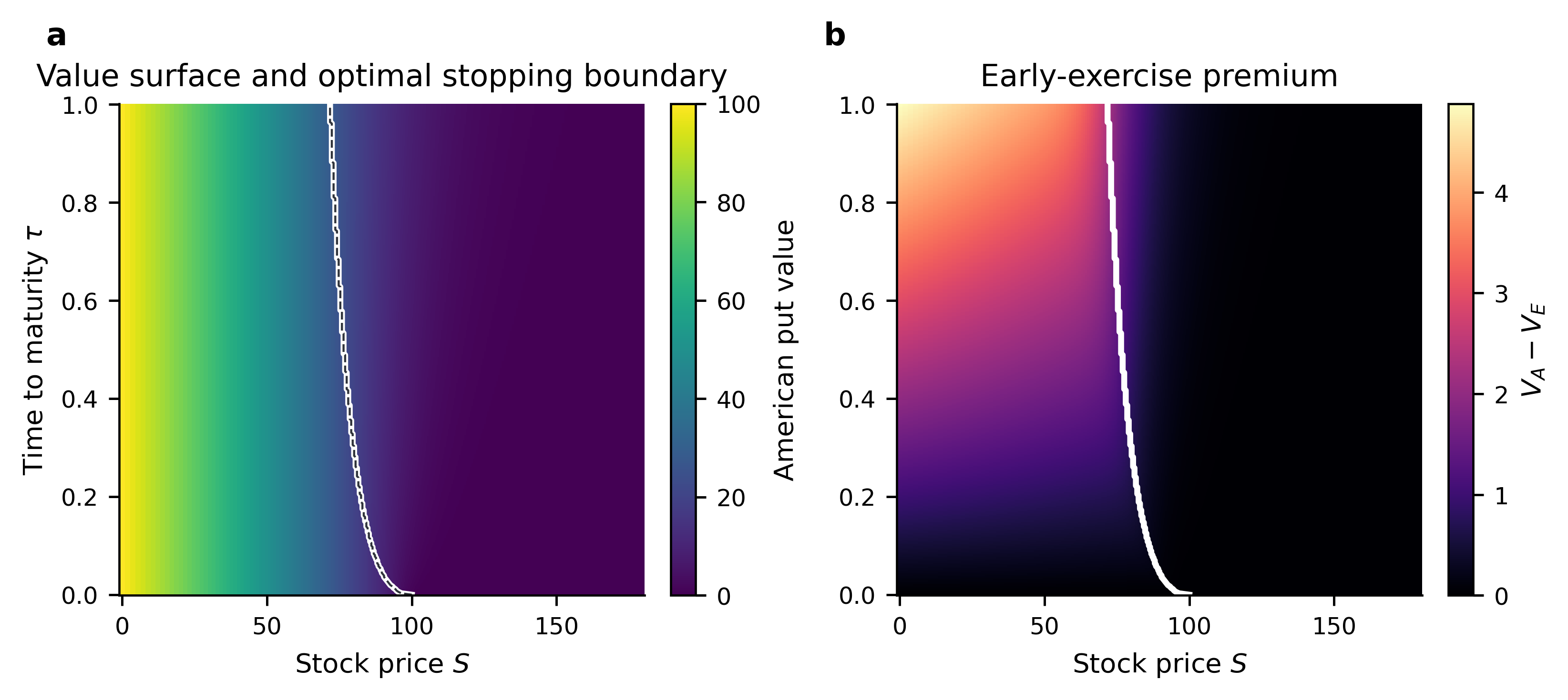
American put value and early-exercise premium over stock price and time, with an optimal-stopping boundary. — **Figure 1.** The value and early-exercise premium share a moving contact boundary. In the configured case, the valuation-date boundary is $S_f(0)\approx71.7972$.

For $S_0=K=100$ , $T=1$ , $r=0.05$ , $q=0.02$ , and $\sigma=0.25$ , the obstacle solver gives $V_A(100,0)\approx8.56494$ . These numbers describe the declared experiment, not a calibrated traded contract.

Why price alone is incomplete

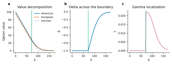
Inside the exercise region, $V=K-S$ , so delta is about $-1$ and gamma about zero. Across the boundary, the continuation value separates smoothly while curvature concentrates near contact.

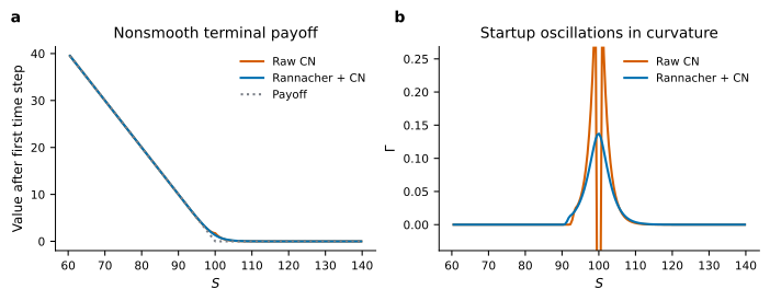
American and European put values, intrinsic payoff, delta, and gamma across the exercise boundary. — **Figure 2.** Value can look stable while gamma remains sensitive near the boundary. Derivatives therefore need their own validation.

The terminal payoff has a kink at the strike. A direct Crank–Nicolson start can transmit it into oscillatory curvature. Two backward-Euler half steps before Crank–Nicolson—the Rannacher treatment—damp that artefact.

Raw Crank-Nicolson and Rannacher-smoothed value and gamma after the first time step. — **Figure 3.** Startup smoothing removes a nonphysical gamma oscillation that a scalar price check could miss.

Solving and auditing the obstacle

On a strike-clustered grid, each time step is a linear complementarity problem:

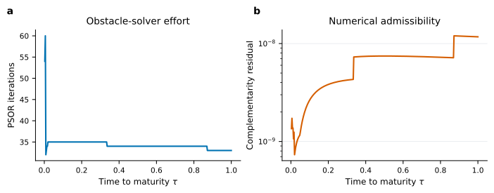
AV^{n+1}\ge b,\qquad V^{n+1}\ge\Phi,\qquad (AV^{n+1}-b)^\top(V^{n+1}-\Phi)=0.

Projected successive over-relaxation combines a Gauss–Seidel update with projection onto $\Phi=(K-S)^+$ . The computation records iteration counts and a residual spanning primal feasibility, dual feasibility, and complementarity.

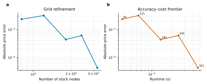
PSOR iteration counts and complementarity residual over time to maturity. — **Figure 4.** The maximum complementarity residual is $1.20\times10^{-8}$ and the maximum PSOR count is 60 for this grid and tolerance.

A small algebraic residual is not enough. Grid refinement compares each finite-difference value with a finer reference and places error beside runtime.

American put price error against stock-grid refinement and runtime. — **Figure 5.** Refinement is not perfectly monotone because the payoff kink and moving contact set interact with the grid, but the finest solution sharply reduces price error.

Three numerical routes

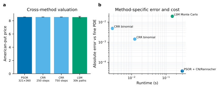
The obstacle PDE, Cox–Ross–Rubinstein trees, and least-squares Monte Carlo answer the same economic question with different error structures. Trees discretise exercise dates; Monte Carlo adds sampling and regression error; the PDE truncates space and time.

Price and error-cost comparison for obstacle PDE, binomial trees, and least-squares Monte Carlo. — **Figure 6.** Agreement across independent routes is stronger evidence than self-consistency inside one solver. Compact axis labels prevent the method names from colliding.

Parameters change both price and policy

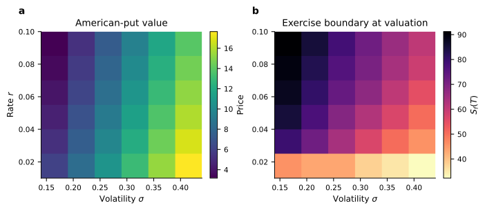
Volatility usually raises option value through convexity, while higher interest rates can make earlier receipt of the strike more attractive. Price and boundary need not move in the same way throughout parameter space.

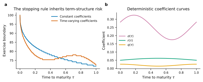
American put price and valuation-date exercise boundary across rates and volatilities. — **Figure 7.** The stopping rule is a policy surface, not a decorative by-product of the scalar price.

The solver also permits deterministic $r(\theta)$ , $q(\theta)$ , and $\sigma(\theta)$ , using midpoint coefficients at each step.

Exercise boundaries under constant and time-varying rates, dividends, and volatility. — **Figure 8.** Similar present-day inputs can imply different stopping paths when their future coefficient curves differ.

What has been verified

The pinned environment passes three automated tests. The complete reproduction regenerates and checksum-validates 34 declared outputs, including all eight figure groups; a quick configuration also succeeds from an empty output directory. Figure titles, panel labels, legends, and method names were visually checked for overlap, and all text is black.

The study establishes reproducibility of this numerical experiment. It does not establish that geometric Brownian motion describes a particular market. Stochastic volatility, jumps, stochastic rates, discrete dividends, transaction costs, liquidity, and calibration uncertainty remain outside scope.

A useful next step is to propagate parameter uncertainty into a distribution over stopping boundaries rather than report one sharp policy. The central lesson is already clear: an American option should be audited as a price, a stopping policy, and a complementarity problem at the same time.

References

Brennan, M. J., & Schwartz, E. S. (1977). The valuation of American put options. The Journal of Finance, 32(2), 449–462. https://doi.org/10.1111/j.1540-6261.1977.tb03284.x
Rannacher, R. (1984). Finite element solution of diffusion problems with irregular data. Numerische Mathematik, 43, 309–327. https://doi.org/10.1007/BF01390130
Longstaff, F. A., & Schwartz, E. S. (2001). Valuing American options by simulation: A simple least-squares approach. The Review of Financial Studies, 14(1), 113–147. https://doi.org/10.1093/rfs/14.1.113
Merton, R. C. (1976). Option pricing when underlying stock returns are discontinuous. Journal of Financial Economics, 3(1–2), 125–144. https://doi.org/10.1016/0304-405X(76)90022-2