When Do Simple Drug-Release Laws Stop Being Enough?

A smooth cumulative-release curve invites a simple question: which equation fits it best? The more useful question is harder: which physical assumptions must be true before that equation is interpretable?

This study places familiar empirical laws beside a spherical diffusion model with finite external volume and clearance. The models are tested on controlled synthetic observations, so the goal is not to recommend a formulation or infer a clinical dose. It is to show where convenient release laws remain informative—and where their apparent simplicity hides transport regimes or non-identifiable parameters.

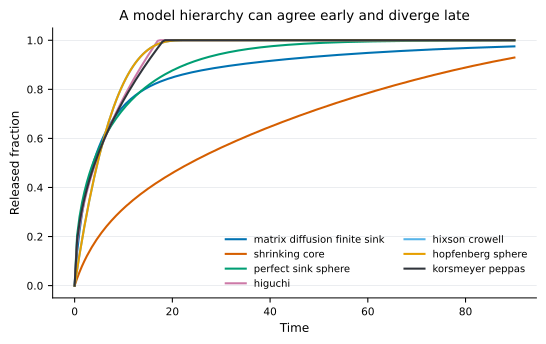
A hierarchy, not a horse race

Several common release relations can be written for the released fraction $F(t)$ :

F_{\mathrm{Higuchi}}(t)=k_H t^{1/2},

F_{\mathrm{Korsmeyer-Peppas}}(t)=k t^n,

F_{\mathrm{Hixson-Crowell}}(t)=1-(1-k_{HC}t)^3,

with a geometry-dependent Hopfenberg form for surface erosion. These are valuable summaries, but their parameters need not map uniquely to diffusion, mass transfer, solubility, or geometry.

The mechanistic model instead follows concentration $C(r,t)$ inside a sphere:

\frac{\partial C}{\partial t} =D\,\frac{1}{r^2}\frac{\partial}{\partial r} \left(r^2\frac{\partial C}{\partial r}\right),

with symmetry at $r=0$ and a finite-transfer boundary at $r=R$ ,

-D\left.\frac{\partial C}{\partial r}\right|_{R} =k_m\,[C(R,t)-C_b(t)].

The bulk concentration $C_b$ evolves with finite volume and clearance, so material that leaves the matrix does not disappear from the mass balance.

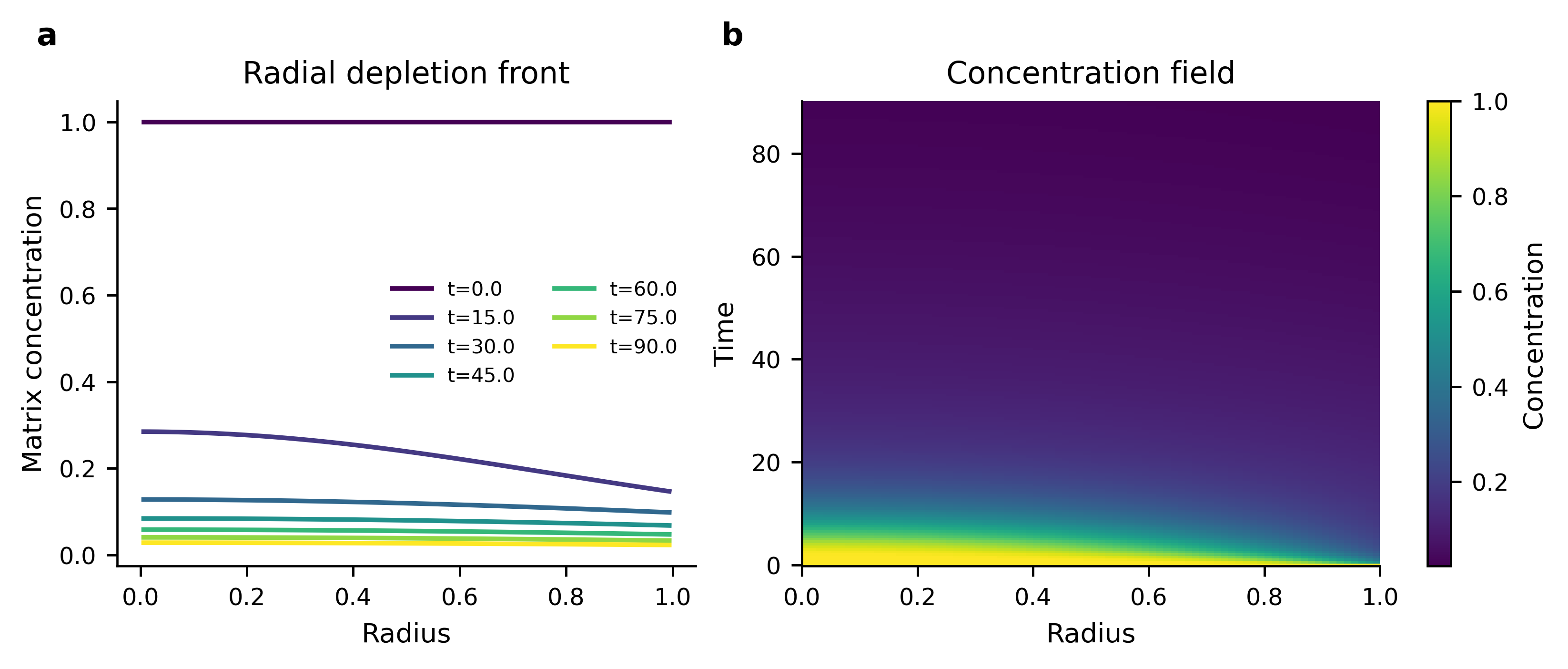
Hierarchy from empirical drug-release laws to a finite-sink spherical diffusion model. — **Figure 1.** Each step adds physical structure and parameters. More mechanism is useful only when the data can constrain it.

The concentration field explains the curve

A cumulative fraction compresses an entire spatial process into one number. Radial profiles reveal the moving depletion layer, the interior reservoir, and the effect of the external sink.

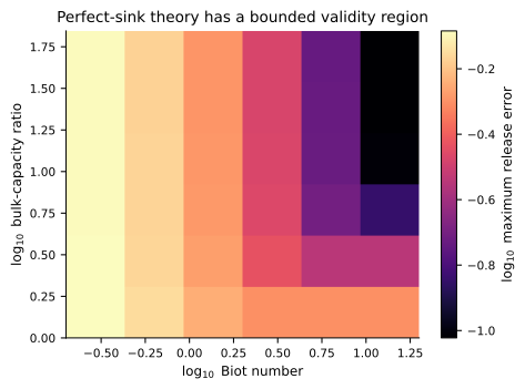
Radial concentration profiles inside a spherical matrix across time, paired with release and bulk concentration. — **Figure 2.** The same cumulative release can arise from different internal concentration fields. The raster format is deliberate for this dense field plot; the remaining diagrams retain vector SVG.

Two dimensionless groups organise the behaviour. A mass-transfer Biot number compares external transfer with internal diffusion,

\mathrm{Bi}_m=\frac{k_mR}{D},

while a capacity ratio compares the matrix inventory with the receiving phase. Low $\mathrm{Bi}_m$ exposes an external-transfer bottleneck; limited capacity weakens the sink and changes late-time release.

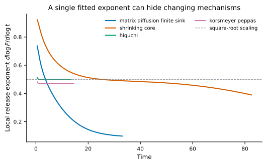
Drug-release regime atlas across mass-transfer Biot number and external capacity ratio. — **Figure 3.** “Diffusion controlled” is not a label that can be assigned from curve shape alone; it depends on where the experiment lies in the transport atlas.

A fitted exponent can drift

For the power law $F=kt^n$ , a local logarithmic slope is

n_{\mathrm{local}}(t)=\frac{d\log F}{d\log t}.

If one fixed mechanism dominated, this exponent would remain nearly constant over its valid interval. In the mechanistic simulation it changes as depletion, external accumulation, and clearance redistribute the limiting resistance.

Local logarithmic drug-release exponent over time for different transport regimes. — **Figure 4.** A single fitted exponent is an average over a window. Moving that window can change the mechanistic story.

Fit quality is evidence, not a verdict

Twenty synthetic observations were generated with declared noise. The candidate models were fitted over a common release interval and compared using residual structure and Akaike information criterion,

\mathrm{AIC}=2k-2\log \hat L.

Observed release, fitted candidate models, residuals, and AIC comparison. — **Figure 5.** The finite-sink PDE has the lowest AIC in the declared experiment, $-179.924$. That result identifies the best candidate here, not a universally superior law.

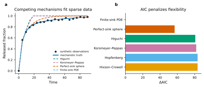
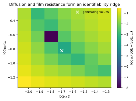
The more mechanistic fit also exposes a common inverse-problem difficulty: $D$ and $k_m$ can trade off. Different parameter pairs generate similar release trajectories, producing a likelihood valley rather than a sharply identified point.

Objective surface over diffusion and mass-transfer parameters showing an identifiability ridge. — **Figure 6.** A narrow residual range does not guarantee individually precise physical parameters. Independent transfer or profile measurements would break the ridge more effectively than more samples at the same times.

Particle-size variation changes the apparent kinetics

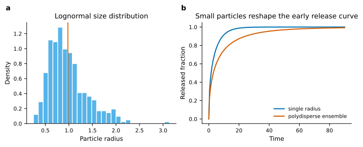
A formulation rarely contains perfectly identical particles. Because diffusion time scales approximately as $R^2/D$ , a distribution of radii becomes a distribution of release times.

Particle-radius distribution and the resulting ensemble drug-release curve compared with a monodisperse model. — **Figure 7.** Polydispersity can broaden the release curve without changing the microscopic transport law. Fitting one effective radius may misattribute heterogeneity to anomalous kinetics.

Numerical conservation is part of the scientific claim

The radial PDE was refined over multiple grid sizes and audited through a closed mass balance. In the default run, the maximum balance error is $3.11\times10^{-13}$ and the final released fraction is $0.9750$ .

Radial-grid convergence and drug mass-balance error for the finite-sink solver. — **Figure 8.** Solver convergence and conservation are reported separately from model fit. A well-fitted curve produced by a leaking discretisation would not be valid evidence.

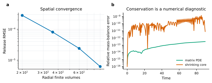
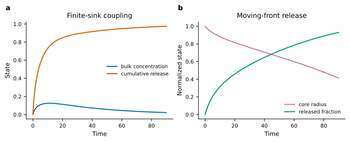
The hierarchy also includes a moving-front or shrinking-core description for dissolution limited by solubility. Comparing it with finite-sink diffusion shows how two plausible mechanisms diverge beyond their shared early-time behaviour.

Finite-sink diffusion and moving-front release predictions with their internal state variables. — **Figure 9.** Early agreement does not imply mechanistic equivalence. Late-time release and internal profiles are stronger discriminators.

What has been verified

The pinned environment passes three automated tests. The complete run regenerates and checksum-validates 41 declared outputs, including nine figure groups. The same pipeline also succeeds from an empty quick-output directory. SVGs are exported directly by the plotting system, preserving the intended visual design without a CairoSVG runtime dependency.

The result supports three conclusions for this declared synthetic experiment:

the finite-sink PDE is the best AIC candidate among those tested;
finite external capacity and mass transfer can make the apparent release exponent time-dependent;
a good mechanistic fit can still leave physical parameters weakly identified.

It does not establish bioavailability, therapeutic equivalence, manufacturing quality, or safety. Those require experimental and clinical evidence outside this model.

Designing a more informative experiment

If only cumulative release is measured, adding more closely spaced time points may yield less information than adding a different observable. A small number of internal concentration profiles, experiments at two external volumes, or independent mass-transfer measurements could rotate and narrow the identifiability ridge.

The practical lesson is not to abandon simple laws. It is to use them at the right level: as compact descriptions until the scientific question requires—and the data can support—a mechanistic explanation.

References

Noyes, A. A., & Whitney, W. R. (1897). The rate of solution of solid substances in their own solutions. Journal of the American Chemical Society, 19(12), 930–934. https://doi.org/10.1021/ja02086a003
Higuchi, T. (1961). Rate of release of medicaments from ointment bases containing drugs in suspension. Journal of Pharmaceutical Sciences, 50(10), 874–875. https://doi.org/10.1002/jps.2600501018
Hixson, A. W., & Crowell, J. H. (1931). Dependence of reaction velocity upon surface and agitation. Industrial & Engineering Chemistry, 23(8), 923–931. https://doi.org/10.1021/ie50260a018
Korsmeyer, R. W., Gurny, R., Doelker, E., Buri, P., & Peppas, N. A. (1983). Mechanisms of solute release from porous hydrophilic polymers. International Journal of Pharmaceutics, 15(1), 25–35. https://doi.org/10.1016/0378-5173(83)90064-9
Hopfenberg, H. B. (1976). Controlled release from erodible slabs, cylinders, and spheres. In Controlled Release Polymeric Formulations. https://doi.org/10.1021/bk-1976-0033.ch003