How Much Tail Risk Does a Gaussian Model Hide?

A Gaussian risk model can be perfectly implemented and still be dangerously calm. The problem is not simply that large returns occur. Financial loss series can combine volatility clustering, asymmetric responses to bad news, heavy-tailed innovations, and occasional jumps. A model that compresses these features into one standard deviation may report a precise number for the wrong tail.

This study creates a controlled stress environment and compares Gaussian EWMA, Gaussian GARCH, Student- $t$ GARCH, filtered historical simulation, and peaks-over-threshold extreme-value methods. The experiment is synthetic: it tests model behaviour, not a portfolio, security, or investment strategy.

The stress environment

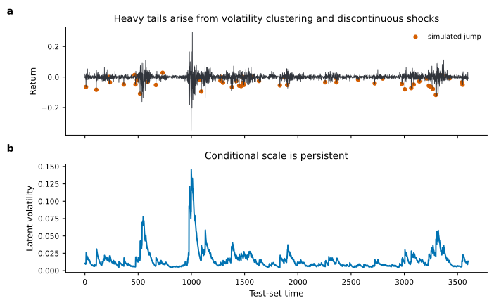
Returns are generated from a leverage-aware volatility process,

r_t=\sigma_t z_t+J_t,

\sigma_t^2 =\omega+\alpha r_{t-1}^2 +\gamma r_{t-1}^2\mathbf 1(r_{t-1}<0) +\beta\sigma_{t-1}^2,

where $z_t$ has Student- $t$ tails and $J_t$ introduces rare negative jumps. The default run contains 7,600 observations, with 3,200 used for fitting and 3,600 for out-of-sample evaluation.

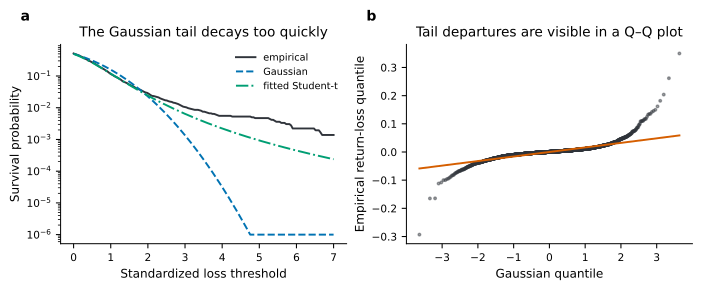
Synthetic returns and latent volatility showing clusters, asymmetric shocks, and negative jumps. — **Figure 1.** Risk changes through time. A single unconditional bell curve cannot express the clustered scale or leverage built into the experiment.

Tail diagnostics test the Gaussian assumption before any forecast score is calculated.

Histogram, quantile plot, mean excess, and tail-index diagnostics for heavy-tailed returns. — **Figure 2.** Deviations in the quantile plot and stable tail diagnostics show why variance alone is an incomplete description of extreme loss.

VaR draws a line; expected shortfall looks beyond it

At confidence level $p$ , value at risk is the loss quantile

\Pr(L_t>\mathrm{VaR}_{p,t}\mid\mathcal F_{t-1})=1-p,

while expected shortfall averages losses beyond that threshold,

\mathrm{ES}_{p,t} =\mathbb E[L_t\mid L_t>\mathrm{VaR}_{p,t},\mathcal F_{t-1}].

VaR therefore asks how often a boundary should be crossed; ES asks how severe a crossing is expected to be.

Out-of-sample losses with time-varying 99 percent VaR forecasts from several models. — **Figure 3.** Forecasts agree in quiet periods and diverge after shocks. Tail assumptions matter most precisely when the risk number is most consequential.

Coverage is necessary, not sufficient

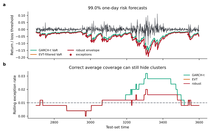
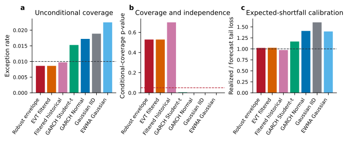
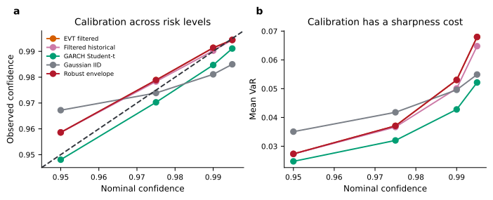
For a nominal 99% VaR, a calibrated model should produce an exception rate near 1%. In the declared run, filtered historical simulation is closest at $0.00972$ . Yet the same count can arise from independent exceptions or from failures clustered after volatility shocks.

The audit therefore separates unconditional coverage, exception independence, and a joint conditional-coverage test.

VaR exception rates and coverage, independence, and conditional-coverage backtests across models. — **Figure 4.** Passing an exception-count check does not prove that forecast dynamics are adequate. Clustering is a distinct failure mode.

Testing one confidence level can also reward a lucky threshold. Calibration curves ask whether forecasts remain aligned across 95%, 97.5%, 99%, and 99.5%.

Observed versus nominal VaR exception rates across multiple confidence levels. — **Figure 5.** A model that is correct at 99% but systematically misses neighbouring levels has not learned the whole tail.

How much risk can the Gaussian assumption conceal?

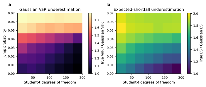
The controlled surface varies Student- $t$ degrees of freedom and jump probability while holding the evaluation rule fixed. Large degrees of freedom approach the Gaussian case; smaller values thicken the tail.

Surface of Gaussian VaR and expected-shortfall underestimation across tail thickness and jump probability. — **Figure 6.** Tail misspecification and jumps reinforce each other. The Gaussian error is not a constant correction factor.

The fitted Student- $t$ GARCH model estimates $\nu\approx4.2685$ . That is far from the Gaussian limit and implies that tail shape is doing substantive work, not merely polishing the fourth decimal place.

Estimated risk has sampling uncertainty

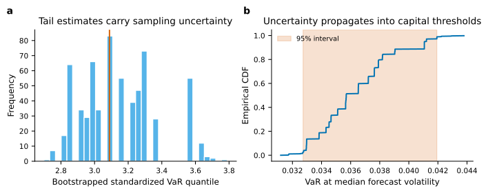
A risk number is itself an estimate. A moving-block bootstrap preserves short-run dependence while resampling the series, producing intervals for both VaR and ES.

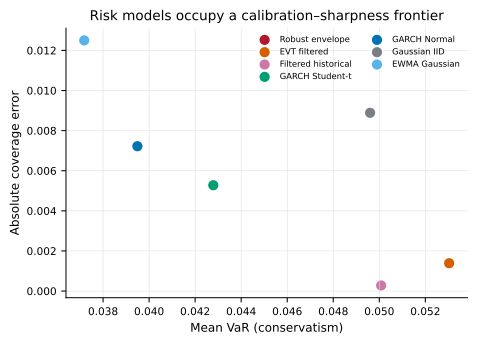
Moving-block bootstrap distributions and intervals for VaR and expected shortfall. — **Figure 7.** Expected shortfall is typically less sharp because it depends on fewer, more extreme observations. Reporting a point estimate alone hides that fragility.

This motivates a second evaluation axis: a model should be calibrated, but its estimates should also be sufficiently sharp to be useful. The risk–sharpness frontier displays that trade-off without cluttered point labels; a separate legend keeps annotations from overlapping.

Risk calibration versus forecast sharpness frontier for the candidate tail models. — **Figure 8.** No single score captures everything. A conservative but noisy forecast and a sharp but miscalibrated forecast fail in different ways.

Dynamics and tails must be checked together

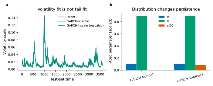
Finally, the fitted conditional scales and innovations reveal whether each model is adapting for the right reason.

Fitted conditional volatility and standardised residual diagnostics for Gaussian and Student-t models. — **Figure 9.** A dynamic scale model can remove volatility clustering while still leaving heavy residual tails. Volatility fit and innovation fit are separate checks.

What has been verified

The pinned environment passes three automated tests. The complete reproduction regenerates and checksum-validates 37 declared outputs, including all nine figure groups; a quick configuration also succeeds from an empty directory. Titles, panel letters, legends, frontier labels, and narrow-screen behaviour were explicitly checked for collisions. All figure text is black.

Within the declared experiment:

filtered historical simulation is closest to the 1% target exception rate;
the fitted Student- $t$ degrees of freedom is about $4.27$ ;
Gaussian underestimation worsens jointly with tail thickness and jump frequency;
calibration, independence, ES severity, and uncertainty give different model rankings.

These statements are properties of a controlled data-generating process. They are not investment advice and do not estimate the risk of any real asset.

The research question that follows

A natural extension is distributional robustness under regime change. Instead of choosing one innovation family, one could form a set of plausible tails and optimise capital or decision rules against their worst calibrated member. Another extension is multivariate: dependence often becomes stronger in stress, so marginally calibrated VaR can still miss joint losses.

The durable lesson is that tail risk is not one number. It is a chain of assumptions about dynamics, distribution, thresholds, exceedance severity, and uncertainty—and every link can be tested.

References

Engle, R. F. (1982). Autoregressive conditional heteroscedasticity with estimates of the variance of United Kingdom inflation. Econometrica, 50(4), 987–1007. https://doi.org/10.2307/1912773
Bollerslev, T. (1986). Generalized autoregressive conditional heteroskedasticity. Journal of Econometrics, 31(3), 307–327. https://doi.org/10.1016/0304-4076(86)90063-1
Glosten, L. R., Jagannathan, R., & Runkle, D. E. (1993). On the relation between the expected value and the volatility of the nominal excess return on stocks. The Journal of Finance, 48(5), 1779–1801. https://doi.org/10.1111/j.1540-6261.1993.tb05128.x
Merton, R. C. (1976). Option pricing when underlying stock returns are discontinuous. Journal of Financial Economics, 3(1–2), 125–144. https://doi.org/10.1016/0304-405X(76)90022-2
McNeil, A. J., & Frey, R. (2000). Estimation of tail-related risk measures for heteroscedastic financial time series. Journal of Empirical Finance, 7(3–4), 271–300. https://doi.org/10.1016/S0927-5398(00)00012-8
Christoffersen, P. F. (1998). Evaluating interval forecasts. International Economic Review, 39(4), 841–862. https://doi.org/10.2307/2527341