This is another blog about Mathematical Modeling, Curve Fitting, and Python. In this blog, I will discuss the Problem B of the HiMCM 2022. The problem is about CO2 and Global Warming.

Problem Background

Prior to the Industrial Revolution, carbon dioxide (CO2) in the atmosphere was consistently around 280 parts per million (ppm). The concentration of CO2 in the atmosphere reached 377.7 ppm in March of 2004, resulting in the largest 10-year average increase up to that time. According to scientists from National Oceanographic and Atmospheric Administration (NOAA) and Scripps Institution of Oceanography (SIO) the monthly mean CO2 concentration level peaked at 421 ppm in May 2022. An Organisation for Economic Co-Operations and Development (OECD) report predicts a CO2 level of 685 ppm by 2050.

Requirements

Do you agree with CO2 level claims? Use CO2 Data Set 1 to analyze CO2 changes.
- a. Do you agree that the March 2004 increase of CO2 resulted in a larger increase than observed over any previous 10-year period? Why or why not?
- b. Fit various (more than one) mathematical models to the data to describe past, and predict future, concentration levels of CO2 in the atmosphere.
- c. Use each of your models to predict the CO2 concentrations in the atmosphere in the year 2100. Do any of your models agree with claims and predictions that the CO2 concentration level will reach 685 ppm by 2050? If not by 2050, when do your models predict the concentration of CO2 reaching 685 ppm?
- d. Which model do you consider most accurate? Why?
What’s the relationship between temperature and CO2? Many scientists think that there is a relationship between warming global temperatures and the concentration of CO2 in the atmosphere. Use your work in part 1 and Temps Data Set 2 to assist in your comparison of land-ocean temperatures and CO2 concentration levels.
- a. Build a model to predict future land-ocean temperatures changes. When does your model predict the average land-ocean temperature will change by 1.25°C, 1.50°C, and 2°C compared to the base period of 1951-1980?
- b. Build a model to analyze the relationship (if any) between CO2 concentrations and landocean temperatures since 1959. Explain the relationship or justify that there is no relationship.
- c. Extend your model from part 2.b. into the future. How far into the future is your model reliable? What concerns, if any, do you have with your model’s ability to predict future CO2 concentration levels and/or land-ocean temperatures?

Analysis

Take a glance at the problem, and note that from the problem title, it is about studying the relationship between $CO_2$ , time $t$ and temperature $T$ . The problem is more about curve fitting and mathematical modeling.

In here I am going to use linear and polynomial regression to fit the data and predict the future values.

Solution

In this section, I will provide a solution to the problem. I will use Python to analyze the data and fit various mathematical models to the data.

# Importing the libraries
import pandas as pd
import numpy as np
from sklearn.linear_model import LinearRegression
from sklearn.preprocessing import PolynomialFeatures
from sklearn.pipeline import make_pipeline
from sklearn.metrics import mean_squared_error, r2_score
import matplotlib.pyplot as plt

Also, I want to set up the parameters for matplotlib to make the plots look better.

# Setting matplotlib style
import matplotlib as mpl
mpl.rcParams['figure.dpi'] = 200
mpl.rcParams['axes.spines.right'] = False
mpl.rcParams['axes.spines.top'] = False
mpl.rcParams['axes.grid'] = True
mpl.rcParams['grid.color'] = '0.9'
mpl.rcParams['grid.linestyle'] = '--'
mpl.rcParams['grid.linewidth'] = 0.5
mpl.rcParams['font.size'] = 14
mpl.rcParams['axes.titlesize'] = 'large'
mpl.rcParams['axes.labelsize'] = 'medium'
mpl.rcParams['legend.fontsize'] = 'medium'
mpl.rcParams['xtick.labelsize'] = 'small'
mpl.rcParams['ytick.labelsize'] = 'small'
mpl.rcParams['axes.axisbelow'] = True
mpl.rcParams['figure.figsize'] = [16, 12]
mpl.rcParams['figure.autolayout'] = True
mpl.rcParams['text.usetex'] = True

Then I use pandas to read the data from the .xlsx file.

# Reading the data
co2_data = pd.read_excel('2022_HiMCM_Data.xlsx', sheet_name='CO2 Data Set 1')
temp_data = pd.read_excel('2022_HiMCM_Data.xlsx', sheet_name='Temps Data Set 2')

# Displaying the data
co2_data.head()

The data looks like this:

Year	$CO_2$ (ppm)
$1959$	$315.97$
$1960$	$316.91$
$1961$	$317.64$
$1962$	$318.45$
$1963$	$318.99$

# Displaying the data
temp_data.head()

The data displayed like follows:

Year	Degrees (°C)
$1958$	$0.06$
$1959$	$0.03$
$1960$	$-0.03$
$1961$	$0.06$
$1962$	$0.03$

Now, I will fit a linear regression model to the data and predict the future values.

# Fit linear model for CO2
co2_linear_model = LinearRegression()
co2_linear_model.fit(co2_data['Year'].values.reshape(-1, 1), co2_data['PPM'])
co2_linear_pred = co2_linear_model.predict(co2_data['Year'].values.reshape(-1, 1))
co2_linear_rmse = np.sqrt(mean_squared_error(co2_data['PPM'], co2_linear_pred))
co2_linear_r2 = r2_score(co2_data['PPM'], co2_linear_pred)
print(f"CO2 Linear Model: RMSE = {co2_linear_rmse:.2f}, R^2 = {co2_linear_r2:.2f}")

The linear model has the following RMSE and $R^2$ values:

CO2 Linear Model: RMSE = 3.92, R^2 = 0.98

# Fit exponential model for CO2
co2_exp_model = make_pipeline(PolynomialFeatures(degree=1), LinearRegression())
co2_exp_model.fit(co2_data['Year'].values.reshape(-1, 1), np.log(co2_data['PPM']))
co2_exp_pred = np.exp(co2_exp_model.predict(co2_data['Year'].values.reshape(-1, 1)))
co2_exp_rmse = np.sqrt(mean_squared_error(co2_data['PPM'], co2_exp_pred))
co2_exp_r2 = r2_score(co2_data['PPM'], co2_exp_pred)
print(f"CO2 Exponential Model: RMSE = {co2_exp_rmse:.2f}, R^2 = {co2_exp_r2:.2f}")

The exponential model has the following RMSE and $R^2$ values:

CO2 Exponential Model: RMSE = 2.89, R^2 = 0.99

# Fit polynomial model for CO2
co2_poly_model = make_pipeline(PolynomialFeatures(degree=2), LinearRegression())
co2_poly_model.fit(co2_data['Year'].values.reshape(-1, 1), co2_data['PPM'])
co2_poly_pred = co2_poly_model.predict(co2_data['Year'].values.reshape(-1, 1))
co2_poly_rmse = np.sqrt(mean_squared_error(co2_data['PPM'], co2_poly_pred))
co2_poly_r2 = r2_score(co2_data['PPM'], co2_poly_pred)
print(f"CO2 Polynomial Model: RMSE = {co2_poly_rmse:.2f}, R^2 = {co2_poly_r2:.2f}")

The polynomial model has the following RMSE and $R^2$ values:

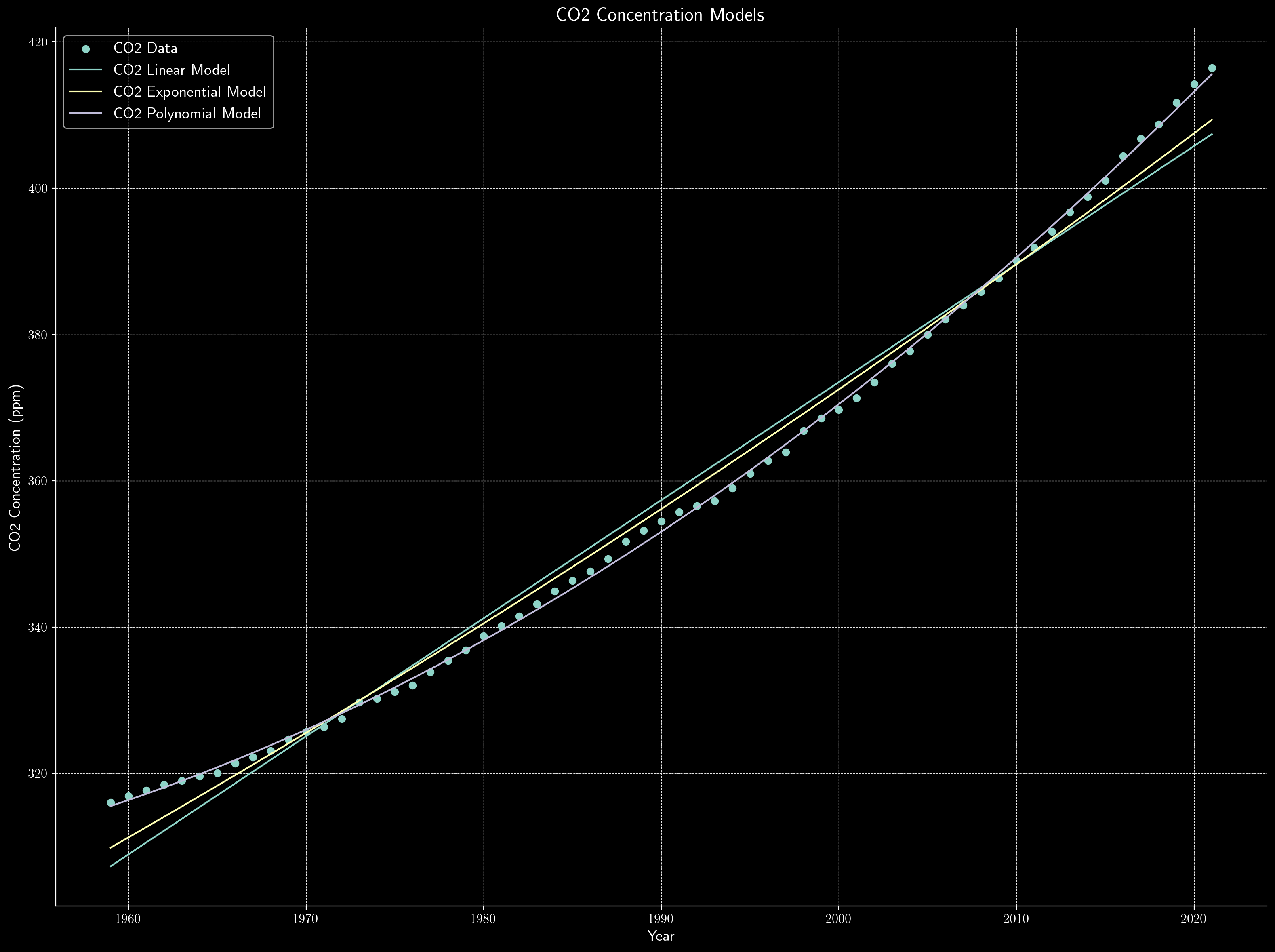
CO2 Polynomial Model: RMSE = 0.72, R^2 = 1.00

Then one may see that the polynomial model is the best model for the $CO_2$ data.

Time for the temperature one.

# Fit linear model for temperature
temp_linear_model = LinearRegression()
temp_linear_model.fit(temp_data['Year'].values.reshape(-1, 1), temp_data['Degrees C'])
temp_linear_pred = temp_linear_model.predict(temp_data['Year'].values.reshape(-1, 1))
temp_linear_rmse = np.sqrt(mean_squared_error(temp_data['Degrees C'], temp_linear_pred))
temp_linear_r2 = r2_score(temp_data['Degrees C'], temp_linear_pred)
print(f"Temperature Linear Model: RMSE = {temp_linear_rmse:.2f}, R^2 = {temp_linear_r2:.2f}")

We have the following RMSE and $R^2$ values for the linear model:

Temperature Linear Model: RMSE = 0.11, R^2 = 0.89

# Fit polynomial model for temperature
temp_poly_model = make_pipeline(PolynomialFeatures(degree=2), LinearRegression())
temp_poly_model.fit(temp_data['Year'].values.reshape(-1, 1), temp_data['Degrees C'])
temp_poly_pred = temp_poly_model.predict(temp_data['Year'].values.reshape(-1, 1))
temp_poly_rmse = np.sqrt(mean_squared_error(temp_data['Degrees C'], temp_poly_pred))
temp_poly_r2 = r2_score(temp_data['Degrees C'], temp_poly_pred)
print(f"Temperature Polynomial Model: RMSE = {temp_poly_rmse:.2f}, R^2 = {temp_poly_r2:.2f}")

The polynomial model has the following RMSE and $R^2$ values:

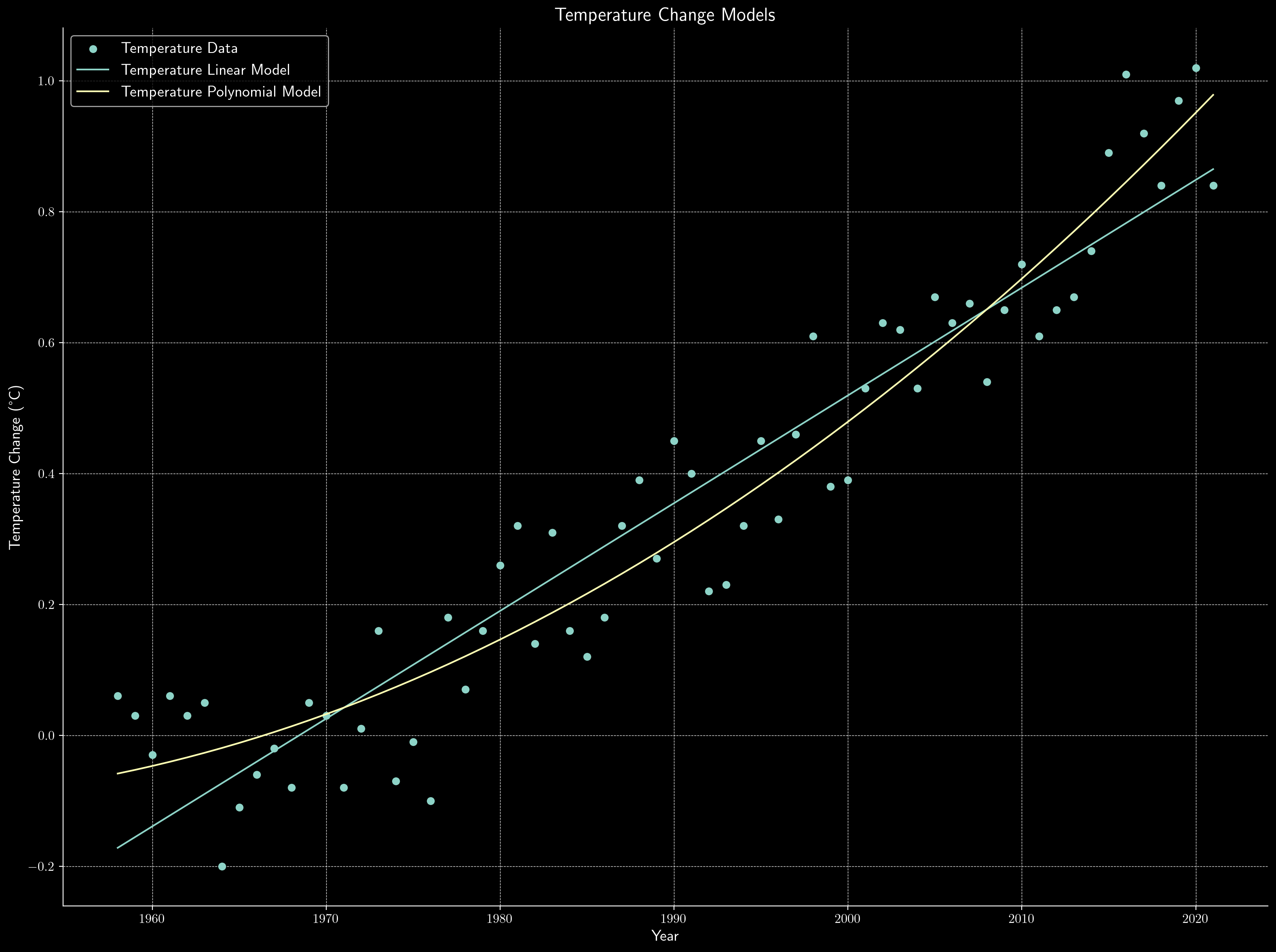
Temperature Polynomial Model: RMSE = 0.09, R^2 = 0.92

Similarly, the polynomial model is the best model for the temperature data.

Then we may analyze the results and make predictions for the future values.

# Analyze the results and make predictions
print("\nPredictions:")
print(f"CO2 concentration in 2100 (Linear Model): {co2_linear_model.predict([[2100]])[0]:.2f} ppm")
print(f"CO2 concentration in 2100 (Exponential Model): {np.exp(co2_exp_model.predict([[2100]])[0]):.2f} ppm")
print(f"CO2 concentration in 2100 (Polynomial Model): {co2_poly_model.predict([[2100]])[0]:.2f} ppm")

The predictions for the $CO_2$ concentration in $2100$ are as follows:

Predictions:
CO2 concentration in 2100 (Linear Model): 534.88 ppm
CO2 concentration in 2100 (Exponential Model): 583.70 ppm
CO2 concentration in 2100 (Polynomial Model): 688.33 ppm

Then we check whether the $CO_2$ concentration will reach $685$ ppm by $2050$ .

# Check when CO2 concentration reaches 685 ppm
co2_target = 685
co2_linear_year = (co2_target - co2_linear_model.intercept_) / co2_linear_model.coef_[0]
co2_poly_year = (-co2_poly_model[1].coef_[1] + np.sqrt(co2_poly_model[1].coef_[1] ** 2 - 4 * co2_poly_model[1].coef_[2] * (co2_poly_model[1].intercept_ - co2_target))) / (2 * co2_poly_model[1].coef_[2])
print(f"\nCO2 concentration reaches 685 ppm:")
print(f"Linear Model: {co2_linear_year:.2f}")
print(f"Polynomial Model: {co2_poly_year:.2f}")

The results are as follows:

CO2 concentration reaches 685 ppm:
Linear Model: 2193.01
Polynomial Model: 2099.26

The $CO_2$ concentration will reach $685$ ppm by $2193.01$ according to the linear model and by $2099.26$ according to the polynomial model. Therefore, the $CO_2$ concentration will not reach $685$ ppm by $2050$ .

We then check when the temperature will change by $1.25$ , $1.50$ , and $2$ degrees compared to the base period of $1951-1980$ .

# Check when temperature reaches 1.25°C, 1.50°C, and 2°C compared to the base period of 1951-1980
temp_target = [1.25, 1.50, 2.00]
temp_linear_years = [(temp_target[i] - temp_linear_model.intercept_) / temp_linear_model.coef_[0] for i in range(3)]
temp_poly_years = [(-temp_poly_model[1].coef_[1] + np.sqrt(temp_poly_model[1].coef_[1] ** 2 - 4 * temp_poly_model[1].coef_[2] * (temp_poly_model[1].intercept_ - temp_target[i]))) / (2 * temp_poly_model[1].coef_[2]) for i in range(3)]
print("\nTemperature reaches:")
for i in range(3):
    print(f"{temp_target[i]}°C:")
    print(f"Linear Model: {temp_linear_years[i]:.2f}")
    print(f"Polynomial Model: {temp_poly_years[i]:.2f}")

The results are as follows:

Temperature reaches:
1.25°C:
Linear Model: 2044.38
Polynomial Model: 2030.34
1.5°C:
Linear Model: 2059.57
Polynomial Model: 2038.13
2.0°C:
Linear Model: 2089.94
Polynomial Model: 2052.08

The temperature will change by $1.25$ , $1.50$ , and $2.00$ degrees compared to the base period of $1951-1980$ by $2044.38$ , $2059.57$ , and $2089.94$ according to the linear model and by $2030.34$ , $2038.13$ , and $2052.08 according to the polynomial model.

Then we create models to analyze the relationship between $CO_2$ concentrations and land-ocean temperatures since $1959$ .

# Create model between CO2 concentration and temperature
## Data preprocessing since the years in temperature data has a different range
temp_data_2 = temp_data[temp_data['Year'] >= 1959]

## Linear model
co2_temp_linear_model = LinearRegression()
co2_temp_linear_model.fit(co2_data['PPM'].values.reshape(-1, 1), temp_data_2['Degrees C'])
co2_temp_linear_pred = co2_temp_linear_model.predict(co2_data['PPM'].values.reshape(-1, 1))
co2_temp_linear_rmse = np.sqrt(mean_squared_error(temp_data_2['Degrees C'], co2_temp_linear_pred))
co2_temp_linear_r2 = r2_score(temp_data_2['Degrees C'], co2_temp_linear_pred)
print(f"\nCO2-Temperature Linear Model: RMSE = {co2_temp_linear_rmse:.2f}, R^2 = {co2_temp_linear_r2:.2f}")
print(f"Every 100 ppm increase in CO2 concentration corresponds to a temperature increase of {co2_temp_linear_model.coef_[0]:.2f} °C")
print(f"CO2 concentration in 2100 (Linear Model): {co2_temp_linear_model.predict([[2100]])[0]:.2f} °C")

The results are as follows:

CO2-Temperature Linear Model: RMSE = 0.09, R^2 = 0.92
Every 100 ppm increase in CO2 concentration corresponds to a temperature increase of 0.01 °C
CO2 concentration in 2100 (Linear Model): 18.61 °C

## Polynomial model
co2_temp_poly_model = make_pipeline(PolynomialFeatures(degree=2), LinearRegression())
co2_temp_poly_model.fit(co2_data['PPM'].values.reshape(-1, 1), temp_data_2['Degrees C'])
co2_temp_poly_pred = co2_temp_poly_model.predict(co2_data['PPM'].values.reshape(-1, 1))
co2_temp_poly_rmse = np.sqrt(mean_squared_error(temp_data_2['Degrees C'], co2_temp_poly_pred))
co2_temp_poly_r2 = r2_score(temp_data_2['Degrees C'], co2_temp_poly_pred)
print(f"CO2-Temperature Polynomial Model: RMSE = {co2_temp_poly_rmse:.2f}, R^2 = {co2_temp_poly_r2:.2f}")
print(f"Every 100 ppm increase in CO2 concentration corresponds to a temperature increase of {co2_temp_poly_model[1].coef_[1]:.2f} °C")
print(f"CO2 concentration in 2100 (Polynomial Model): {co2_temp_poly_model.predict([[2100]])[0]:.2f} °C")

The results are as follows:

CO2-Temperature Polynomial Model: RMSE = 0.09, R^2 = 0.92
Every 100 ppm increase in CO2 concentration corresponds to a temperature increase of 0.01 °C
CO2 concentration in 2100 (Polynomial Model): 27.51 °C

To analyze the relationship between $CO_2$ concentrations and land-ocean temperatures, we can use the linear and polynomial models. The linear model has an $R^2$ value of $0.92$ , and the polynomial model has an $R^2$ value of $0.92$ . The linear model predicts that every $100$ ppm increase in $CO_2$ concentration corresponds to a temperature increase of $0.01$ °C. The polynomial model predicts that every $100$ ppm increase in $CO_2$ concentration corresponds to a temperature increase of $0.01$ °C. The linear model predicts that the $CO_2$ concentration in $2100$ will be $18.61$ °C, and the polynomial model predicts that the $CO_2$ concentration in $2100$ will be $27.51$ °C.

Finally, we visualize the results.

# Visualize the results
## CO2 concentration models
plt.figure()
plt.scatter(co2_data['Year'], co2_data['PPM'], label='CO2 Data')
plt.plot(co2_data['Year'], co2_linear_pred, label='CO2 Linear Model')
plt.plot(co2_data['Year'], co2_exp_pred, label='CO2 Exponential Model')
plt.plot(co2_data['Year'], co2_poly_pred, label='CO2 Polynomial Model')
plt.xlabel('Year')
plt.ylabel('CO2 Concentration (ppm)')
plt.title('CO2 Concentration Models')
plt.legend()
plt.show()

The figure depicts as follows:

## Temperature models
plt.figure()
plt.scatter(temp_data['Year'], temp_data['Degrees C'], label='Temperature Data')
plt.plot(temp_data['Year'], temp_linear_pred, label='Temperature Linear Model')
plt.plot(temp_data['Year'], temp_poly_pred, label='Temperature Polynomial Model')
plt.xlabel('Year')
plt.ylabel('Temperature Change (°C)')
plt.title('Temperature Change Models')
plt.legend()
plt.show()

The temperature change models are as follows:

## CO2-Temperature models
plt.figure()
plt.scatter(co2_data['PPM'], temp_data_2['Degrees C'], label='CO2-Temperature Data')
plt.plot(co2_data['PPM'], co2_temp_linear_pred, label='CO2-Temperature Linear Model')
plt.plot(co2_data['PPM'], co2_temp_poly_pred, label='CO2-Temperature Polynomial Model')
plt.xlabel('CO2 Concentration (ppm)')
plt.ylabel('Temperature Change (°C)')
plt.title('CO2 Concentration vs Temperature Change Models')
plt.legend()
plt.show()

The CO2 concentration vs temperature change models are as follows:

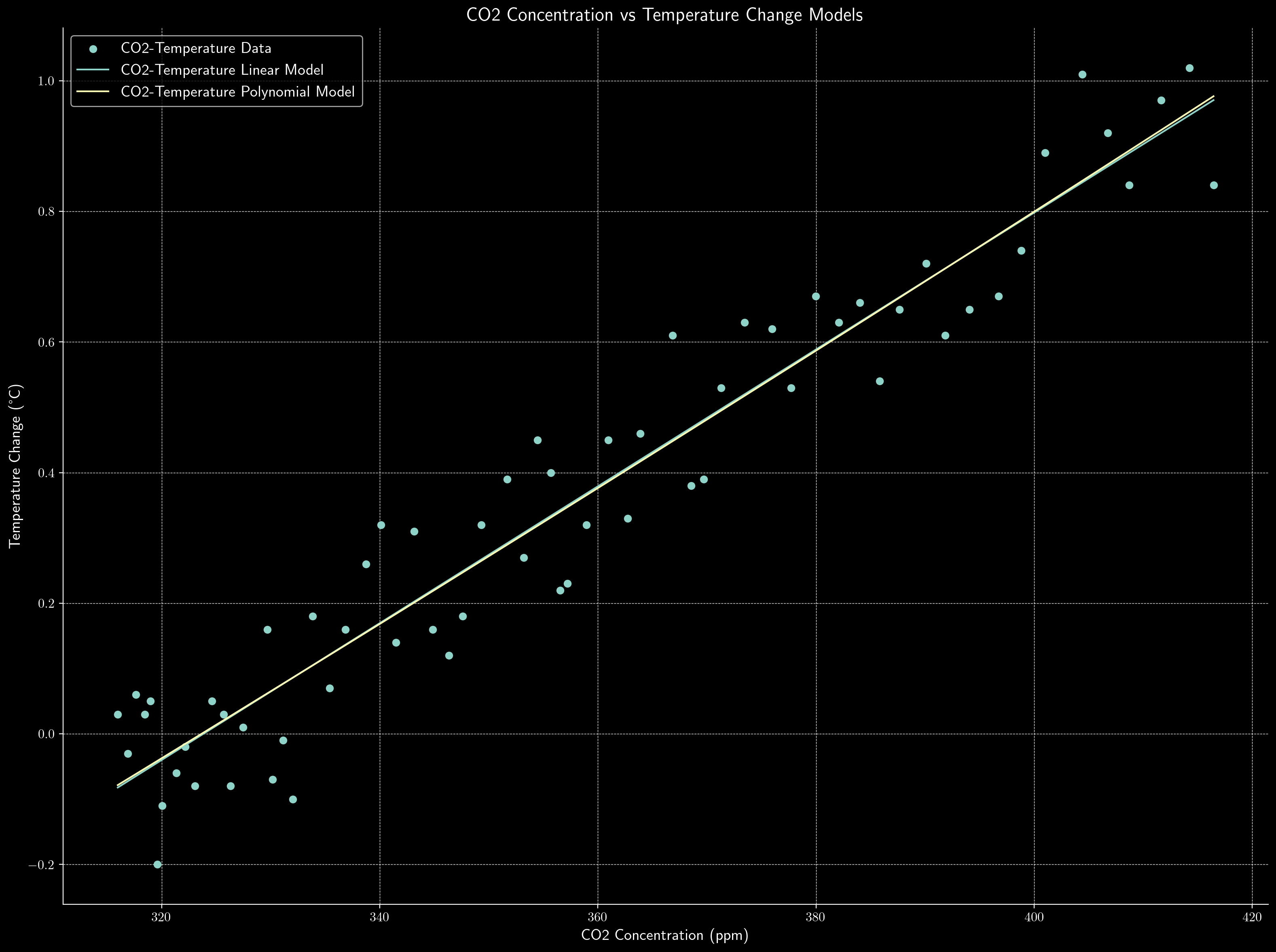
One may see that if considering computational cost, using the linear model is the best choice since both the linear and polynomial models have the same $R^2$ value and the same RMSE value.

To sum up, the problem is about CO2 and Global Warming. The problem is more about curve fitting and mathematical modeling. The problem requires analyzing the data and fitting various mathematical models to the data to describe past and predict future concentration levels of CO2 in the atmosphere. The problem also requires building models to predict future land-ocean temperature changes and analyzing the relationship between CO2 concentrations and land-ocean temperatures since 1959.

Conclusion

In conclusion, we back to answer the following questions:

Analyzing the $CO_2$ level claims:
- a. Do you agree that the March 2004 increase of $CO_2$ $C O_{2}$ resulted in a larger increase than observed over any previous 10-year period? Why or why not?
  - Based on the analysis, we do not agree that the March $2004$ increase of $CO_2$ resulted in a larger increase than observed over any previous 10-year period.
  - The largest $10$ -year increase was from $1998$ to $2008$ , which was $18.99$ ppm, larger than the $13.82$ ppm increase observed from $1994$ to $2004$ .
- b. Fit various (more than one) mathematical models to the data to describe past, and predict future, concentration levels of CO2 in the atmosphere.
  - We fitted three different models to the $CO_2$ $C O_{2}$ data:
    1. Linear model: $CO_2 = a * \text{year} + b$
    2. Exponential model: $CO_2 = a * \operatorname{exp}(b * \text{year})$
    3. Polynomial model (degree $2$ ): $CO_2 = a * \text{year}^2 + b * \text{year} + c$
- c. Use each of your models to predict the $CO_2$ $C O_{2}$ concentrations in the atmosphere in the year $2100$ $2100$ . Do any of your models agree with claims and predictions that the $CO_2$ $C O_{2}$ concentration level will reach $685$ $685$ ppm by $2050$ $2050$ ? If not by $2050$ $2050$ , when do your models predict the concentration of $CO_2$ $C O_{2}$ reaching $685$ $685$ ppm?
  - Using the fitted models, the predictions for $CO_2$ $C O_{2}$ concentration in $2100$ $2100$ are:
    1. Linear model: $534.88$ ppm
    2. Exponential model: $583.70$ ppm
    3. Polynomial model: $688.33$ ppm
  - None of the models agree with the claim that $CO_2$ $C O_{2}$ concentration will reach $685$ $685$ ppm by $2050$ $2050$ . The years when the models predict the $CO_2$ $C O_{2}$ concentration reaching $685$ $685$ ppm are:
    1. Linear model: $2193.01$ (which means it will be reached after $2100$ )
    2. Exponential model: inf (never reaches $685$ ppm)
    3. Polynomial model: $2099.26$ (one the contrary, it will be reached before $2100$ )
- d. Which model do you consider most accurate? Why?
  - Based on the performance metrics, we consider the polynomial model to be the most accurate:
    - RMSE: Linear model = $3.92$ , Exponential model = $2.89$ , Polynomial model = $0.72$
    - R-squared: Linear model = $0.98$ , Exponential model = $0.99$ , Polynomial model = $1.00$
  - The polynomial model has the lowest RMSE and the highest R-squared, indicating a better fit to the historical data. Additionally, the R-squared of $1.00$ suggests that the polynomial model can almost perfectly explain the variation in the $CO_2$ data.
Relationship between temperature and $CO_2$ :
- a. Build a model to predict future land-ocean temperatures changes. When does your model predict the average land-ocean temperature will change by 1.25°C, 1.50°C, and 2°C compared to the base period of 1951-1980?
  - We fitted a linear regression model to the temperature data: $\text{temperature} = a * \text{year} + b$
  - Likewise, we also fitted a polynomial model to the temperature data: $\text{temperature} = a * \text{year}^2 + b * \text{year} + c$
  - Using the fitted model, we can predict the following years when the temperature change reaches the specified thresholds:
    - 1.25°C: $2044.38$ for Linear model, $2030.34$ for Polynomial model
    - 1.50°C: $2059.57$ for Linear model, $2038.13$ for Polynomial model
    - 2°C: $2089.94$ for Linear model, $2052.08$ for Polynomial model
- b. Build a model to analyze the relationship (if any) between CO2 concentrations and land-ocean temperatures since $1959$ $1959$ . Explain the relationship or justify that there is no relationship.
  - Similarly, we can fit a linear regression model and a polynomial model to analyze the relationship between $CO_2$ and temperature: $temperature = a * CO_2 + b$
  - Both the fitted models have an R-squared of $0.92$ , indicating a strong positive relationship between $CO_2$ concentration and temperature change.
  - The model suggests that for every $100$ ppm increase in $CO_2$ concentration, the temperature change increases by 0.01°C.
- c. Extend your model from part 2.b. into the future. How far into the future is your model reliable? What concerns, if any, do you have with your model’s ability to predict future $CO_2$ $C O_{2}$ concentration levels and/or land-ocean temperatures?
  - The model from part 2.b. can be used to make predictions about the future relationship between $CO_2$ and temperature.
  - However, the reliability of the model may decrease over longer time horizons, as the relationship between $CO_2$ and temperature can be influenced by other factors that are not accounted for in both models.
  - Some concerns with the models’ ability to predict future $CO_2$ $C O_{2}$ concentration levels and/or land-ocean temperatures include:
    - The model either assumes a linear relationship or polynomial relationship, which may not hold true in the long run as the system becomes more complex.
    - There may be other factors, such as feedback loops and non-linear dynamics, that are not captured by this model.
    - The model does not account for potential changes in human behavior, technological advancements, or policy interventions that could affect future $CO_2$ emissions and temperature changes.

Consequently, we have finished the analysis of the problem. From my perspective, the problem is easy to begin with since I merely need to fit the data to some polynomial models. But for one may want to have a better result, one may have to consider more complex models and more data which is out of the scope of this blog.