When the Fit Is Not the Model

A curve can pass almost perfectly through the data and still leave the mechanism unresolved.

This is one of the most consequential distinctions in mathematical modeling. Fitting asks whether some parameter vector reproduces the observations. Identification asks whether the observations distinguish that vector from other scientifically different possibilities. A small residual answers the first question; it does not answer the second.

The distinction matters whenever parameters carry interpretation. A fitted rate may be reported as a biological timescale, an infrastructure failure intensity, or the strength of a behavioural response. If many parameter combinations reproduce the same observable curve, the decimal places returned by an optimizer are not measurements of those quantities. They are coordinates of one acceptable solution.

The accompanying identifiability laboratory makes that problem visible through a deliberately small inverse problem. It is not a substitute for a full structural or profile-likelihood analysis. Its purpose is to show why an excellent fit can be the beginning of an inquiry rather than its conclusion.

A ridge hidden behind one optimum

Consider the Michaelis–Menten response

y(S)=\frac{V_{\max}S}{K_m+S}.

The parameter $V_{\max}$ controls the saturation level, while $K_m$ is the substrate level at which the response reaches half of that level. If measurements extend well beyond $K_m$ , the curve contains evidence about both its initial rise and its plateau. If every observation lies at low substrate, then

y(S)\approx \frac{V_{\max}}{K_m}S \qquad \text{when } S\ll K_m.

In that regime the data primarily identify the ratio $V_{\max}/K_m$ . Increasing both parameters together can leave the observed slope almost unchanged. The loss surface therefore develops an elongated low-loss ridge.

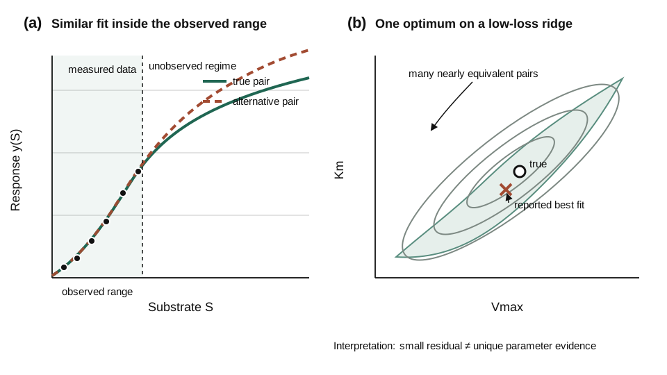
Two-panel schematic showing two parameter curves that agree within the measured substrate range but diverge outside it, alongside an elongated parameter-loss ridge. — **Figure 1.** A close fit can conceal weak parameter evidence. In panel (a), the solid and dashed curves are almost indistinguishable where data exist but separate in the unobserved regime. Panel (b) shows why one reported optimum does not remove the surrounding ridge of nearly equivalent parameter pairs.

The two panels show the same information failure in output space and parameter space. The observed curve constrains a direction across the ridge much more strongly than it constrains movement along the ridge. Reporting only the best point hides that anisotropy.

An optimizer normally returns one point on that surface. The interactive heatmap shows the surrounding surface as well. The circle marks the parameter pair that generated the synthetic observations; the cross marks the best pair on the search grid. Dark cells are alternative pairs with similar mean squared error.

Three controls change the information supplied to the fit:

Maximum observed substrate determines whether the data reach the bending and saturation regions.
Observation noise changes how readily neighbouring curves can be distinguished.
Number of measurements adds replication across the selected range, but does not necessarily add a new kind of information.

The third point is easy to miss. Thirty measurements within the same narrow linear regime may reduce random error while preserving the parameter ridge. One carefully placed high-substrate measurement can be more informative than many additional points where all candidate curves behave alike.

Structural and practical identifiability are different questions

Structural identifiability concerns the model and observation process under ideal information. In simplified terms, it asks whether perfect, noise-free observations could uniquely recover the parameters. If two parameter vectors generate exactly the same observable output for all admissible inputs, no improvement in measurement precision can separate them. The model must be reparameterised, a new quantity must be observed, or a different input must be applied.

Practical identifiability concerns the experiment actually performed. A structurally identifiable model can remain practically non-identifiable because observations are sparse, noisy, restricted to an uninformative time window, or insensitive to one parameter. Raue and colleagues formalised a profile-likelihood approach that exposes both flat parameter relationships and confidence regions that remain unbounded under finite data. Wieland and colleagues later emphasised that practical identifiability should not be reduced to a local covariance calculation around one optimum.

The interactive example illustrates only the practical side. The displayed ridge arises because the synthetic experiment does not sufficiently excite the saturating part of a structurally identifiable response. It would be incorrect to look at that heatmap and declare the Michaelis–Menten form structurally non-identifiable in general.

Why a Hessian can look more certain than the problem

A common uncertainty calculation approximates the loss surface by a quadratic near the optimum. This local approximation is attractive because the inverse Hessian can be interpreted as a parameter covariance matrix under suitable assumptions.

The approximation becomes fragile when the surface is strongly curved, asymmetric, bounded, multimodal, or nearly flat over a long direction. A narrow quadratic fitted to one section of a ridge can miss distant parameter values that still fit acceptably. Reparameterisation can also change the apparent local geometry even though the underlying information has not changed.

Profile likelihood takes a more global view. To profile one parameter, fix it at a sequence of values and re-optimise all remaining parameters. The resulting curve asks how much fit must be sacrificed when that parameter is forced away from its optimum. A profile that never crosses the selected confidence threshold in one direction indicates that the data do not provide a finite bound in that direction under the model and likelihood assumptions.

No uncertainty method removes the need to inspect the observation model. If the noise distribution, censoring process, measurement scale, or experimental input is wrong, a mathematically precise interval can still answer the wrong question.

Turn non-identifiability into an experimental design problem

An identifiability diagnosis becomes useful when it changes what is measured next. A disciplined workflow is:

Define the parameter or prediction that matters scientifically.
Check structural identifiability for the specified inputs and outputs.
Fit the model with held-out checks and inspect global parameter uncertainty.
Find where candidate parameter sets make different predictions.
Place the next measurement or intervention in that discriminating region.

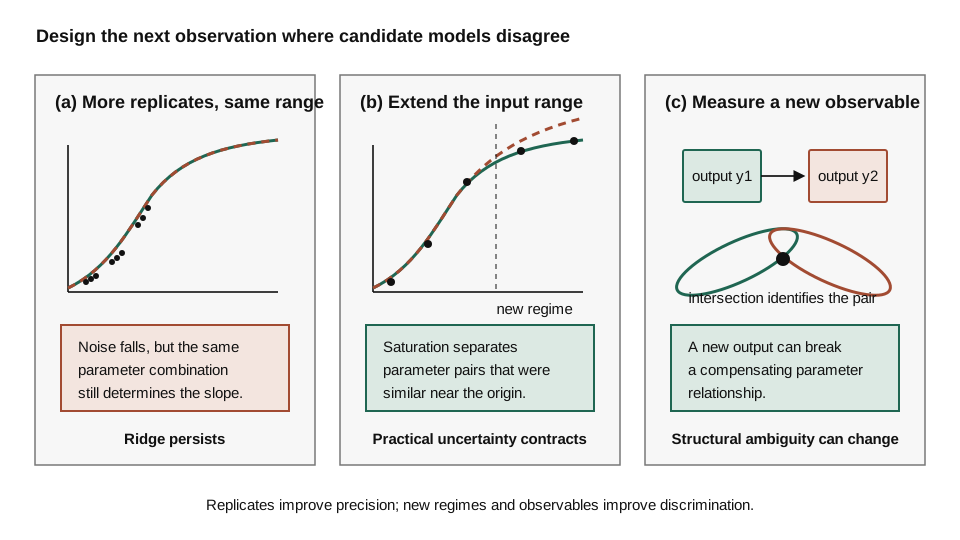
Three-panel comparison of repeated measurements in the same range, measurements extended into a discriminating range, and measurement of a new observable. — **Figure 2.** Three responses to weak identifiability are not equivalent. Replication in the same regime improves precision but can preserve the ridge; extending the input range separates previously similar curves; a genuinely new observable can alter the structural information available to the inverse problem.

The design implication is specific: add information where admissible explanations disagree, not merely where measurement is convenient. More data and more identifying data are different resources.

For the saturation model, the last step suggests extending the substrate range rather than concentrating every new replicate near the origin. For a dynamical system, it may suggest sampling earlier transients, measuring an additional state, or applying a time-varying input. Tools such as STRIKE-GOLDD 4.0 automate structural identifiability and observability tests for broad classes of nonlinear ODE models, but the result still has to be translated into a feasible experiment.

This also changes how models should be simplified. If only a parameter combination is identifiable, that combination may be the scientifically honest quantity to estimate. Fixing one weakly informed parameter at a literature value can make computation easier, but it transfers uncertainty from the data analysis into an assumption. That choice should be visible in the final claim.

A research programme rather than a diagnostic checkbox

The laboratory suggests several studies that go beyond demonstrating a ridge.

One direction is cost-aware experimental design. Given candidate measurement times or substrate levels with different costs, choose the smallest design that bounds the parameter or prediction of interest. The objective need not be a generic determinant of the Fisher information matrix; it can target the width of a profile-likelihood interval or disagreement between plausible models.

A second direction is identifiability under model discrepancy. Classical analyses assume that one candidate model generated the data. Real mechanisms are approximate. A study can test whether a design that identifies parameters under the nominal model remains informative when an omitted process perturbs the observations.

A third direction is prediction-focused identifiability. Parameters can be poorly determined while a particular forecast remains stable, or parameter estimates can look precise while extrapolated predictions diverge. The research question then shifts from “Can every parameter be recovered?” to “Which decisions or forecasts are invariant across the empirically admissible parameter set?”

These questions are especially relevant for student research because they join mathematical analysis, computation, and experimental reasoning. They also reward negative results. Showing that a proposed measurement cannot distinguish two mechanisms is useful evidence when the conclusion leads to a better design.

What this demonstration does not establish

The browser experiment uses deterministic pseudo-noise, a finite parameter grid, mean squared error, and a known two-parameter response. The “near-optimal” count is a visual diagnostic, not a confidence region. It does not account for correlated errors, parameter bounds selected from prior information, model discrepancy, multiple outputs, or uncertainty in the substrate values.

Most importantly, identifiability is conditional on a specified model, input, observation function, and data regime. A parameter is not simply identifiable or non-identifiable in isolation. The claim must name the information structure under which it is made.

Conclusion

A close fit is evidence that a model can reproduce the observations. It is not evidence that the fitted mechanism is unique.

The practical response is not to distrust optimisation. It is to place optimisation inside a larger inferential workflow: inspect the loss geometry, distinguish structural from practical limitations, report parameter combinations when they are what the data support, and design new measurements where plausible explanations disagree.

The most useful question after fitting may therefore be: what observation would make this result harder to imitate?

References

Raue, A., Kreutz, C., Maiwald, T., Bachmann, J., Schilling, M., Klingmüller, U., & Timmer, J. (2009). Structural and practical identifiability analysis of partially observed dynamical models by exploiting the profile likelihood. Bioinformatics, 25(15), 1923–1929. https://doi.org/10.1093/bioinformatics/btp358
Wieland, F.-G., Hauber, A. L., Rosenblatt, M., Tönsing, C., & Timmer, J. (2021). On structural and practical identifiability. Current Opinion in Systems Biology, 25, 60–69. https://doi.org/10.1016/j.coisb.2021.03.005
Díaz-Seoane, S., Rey Barreiro, X., & Villaverde, A. F. (2023). STRIKE-GOLDD 4.0: user-friendly, efficient analysis of structural identifiability and observability. Bioinformatics, 39(1), btac748. https://doi.org/10.1093/bioinformatics/btac748
Kreutz, C., Raue, A., Kaschek, D., & Timmer, J. (2013). Profile likelihood in systems biology. FEBS Journal, 280(11), 2564–2571. https://doi.org/10.1111/febs.12276