A Decision That Survives the Shift

An optimal decision can be a precise answer to a distribution that will not recur.

Demand forecasts shift, sensor populations change, travel behaviour adapts, and rare events remain rare in the calibration sample. A stochastic optimisation model may represent the observed distribution carefully and still select a decision that is fragile to modest probability error. The problem is intensified by optimisation itself: among many candidate decisions, the procedure tends to favour one that exploits the particular sample used to estimate the objective.

Distributionally robust optimisation (DRO) changes the question. Instead of assuming one known probability distribution, it considers a set of plausible distributions and minimises the worst expected cost inside that set:

\min_{q\in\mathcal Q}\;\sup_{p\in\mathcal P(\rho)}\mathbb E_p[c(q,D)].

The robust-decision laboratory applies this idea to a finite capacity problem. It shows the benefit and the price of ambiguity aversion without presenting robustness as a free guarantee.

Nominal, robust, and distributionally robust are not synonyms

A nominal stochastic model selects the decision that minimises expected cost under one distribution $p_0$ :

q_{\text{nom}}\in\arg\min_q \mathbb E_{p_0}[c(q,D)].

Classical robust optimisation instead protects against values of the uncertain quantity in a set, often without attaching probabilities to them. DRO protects against probability distributions in an ambiguity set $\mathcal P$ . This middle position retains expected-cost reasoning while acknowledging that the distribution itself is uncertain.

The distinction matters because the ambiguity set encodes what “plausible shift” means. A moment set protects against distributions sharing selected means or variances. A Wasserstein ball limits the transport cost required to move probability mass from an empirical distribution. A divergence ball limits a statistical discrepancy. The interactive model uses total variation distance on a fixed set of five demand values.

No ambiguity set is automatically correct. It is a modelling object whose geometry should match the data-generating uncertainty and the decision’s failure modes.

A finite capacity problem

The laboratory uses demand states

D\in\{40,55,70,85,100\}

with nominal probabilities $(0.1,0.2,0.4,0.2,0.1)$ . Capacity $q$ incurs asymmetric piecewise-linear cost,

c(q,D)=c_u(D-q)_+ + c_o(q-D)_+,

where $c_u$ is the shortage cost and $c_o$ is the overage cost. A higher shortage penalty favours more capacity; a higher overage penalty discourages unused capacity.

The ambiguity set contains probability vectors within total variation radius $\rho$ of the nominal vector:

\mathcal P(\rho)=\left\{p:\frac12\sum_s|p_s-p_{0s}|\leq\rho,\;p_s\geq0,\;\sum_s p_s=1\right\}.

For any fixed capacity, the worst distribution moves probability mass away from low-cost demand states and toward high-cost states until the movement budget is exhausted. Because the support is finite, this inner maximisation can be solved exactly by a small linear programme; the browser implementation uses the equivalent greedy mass-transfer calculation for this one-dimensional cost vector.

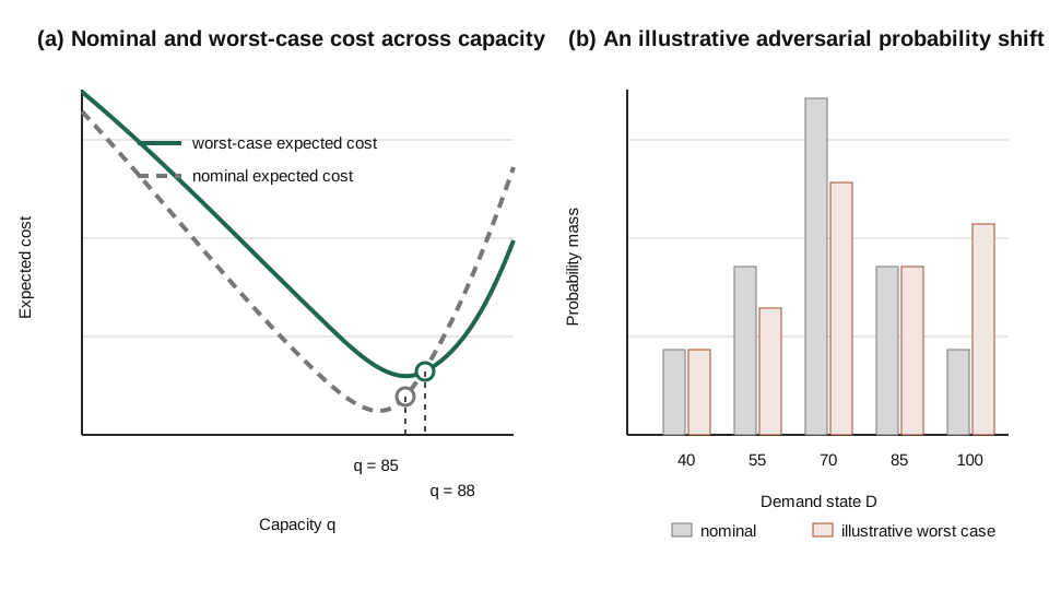
Two-panel schematic comparing nominal and worst-case expected-cost curves across capacity and showing probability mass shifted toward a costly high-demand state. — **Figure 1.** The outer and inner DRO problems are linked. Panel (a) shows illustrative nominal and worst-case expected-cost curves whose minima select different capacities. Panel (b) shows the corresponding stress logic: probability mass is moved away from relatively inexpensive states and toward a costly demand state within the ambiguity budget.

Figure 1 separates two objects that are easily conflated. The upper curve is a decision criterion, while the adversarial probability vector is the distribution attaining that criterion for a fixed decision. Neither should be read as a forecast that the next period will follow the worst case.

The ambiguity radius is a scientific parameter

At $\rho=0$ , the ambiguity set contains only the nominal distribution, so the two optimisation problems coincide. As $\rho$ grows, the worst-case curve rises and may favour a different capacity. The robust solution normally shifts toward protection against the more expensive tail, though the direction depends on the cost asymmetry and support.

It is tempting to move the radius until the model produces a reassuring decision. That reverses the evidential logic. The radius should be calibrated or stress-tested using information not selected to support the final answer.

Possible calibration strategies include concentration bounds, held-out likelihood or coverage, bootstrap variation, known sampling error, or domain scenarios agreed before optimisation. Mohajerin Esfahani and Kuhn show how Wasserstein ambiguity sets can support tractable reformulations and finite-sample performance guarantees under stated assumptions. Those guarantees do not transfer automatically to a different distance, radius rule, dependent dataset, or cost function.

A practical report should therefore show a radius path rather than one preferred value. If the decision changes repeatedly under tiny radius adjustments, the model is telling the analyst that the recommendation depends on fine probability distinctions the data may not support.

The price of robustness needs two ledgers

The laboratory reports a nominal price of robustness:

\mathbb E_{p_0}[c(q_{\text{rob}},D)]- \mathbb E_{p_0}[c(q_{\text{nom}},D)].

This quantity measures how much nominal expected performance is surrendered by using the robust decision. It is useful, but it is only one ledger. The second ledger evaluates both decisions under plausible shifted or held-out distributions. A robust decision is worthwhile when its out-of-distribution loss reduction justifies its nominal premium.

The worst-case objective alone cannot establish that balance empirically. An ambiguity set may be too small and miss relevant shifts, or too large and produce a decision dominated by implausible distributions. Recent work continues to develop ambiguity sets that represent richer information while controlling conservatism. For example, Chen and colleagues introduce moment-dispersion ambiguity to represent location, dispersion, support, and aspects of dependence, and compare its decisions with moment and Wasserstein alternatives in data-limited experiments.

The relevant question is therefore not “Is DRO conservative?” but “Conservative against which shifts, at what nominal cost, and with what empirical calibration?”

A stronger research design

The browser example can become an academic computational study through a predeclared evaluation protocol.

Begin with several data-generating families that agree near the observed sample but differ in tail weight, skewness, dependence, or regime change. Estimate a nominal distribution from training samples of varying size. Construct competing ambiguity sets using only the training data. Select the decision under each method, then evaluate it on large independent test samples from both nominal and shifted families.

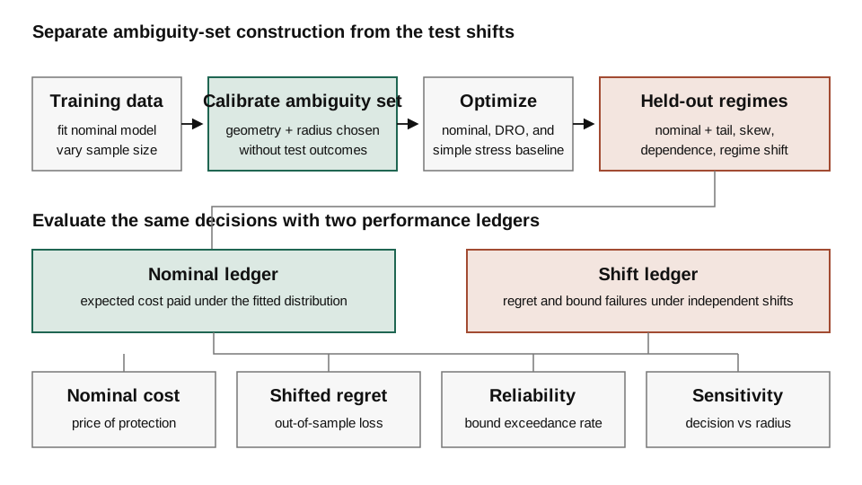
Validation workflow separating training data, ambiguity-set calibration, optimization, and held-out regime tests, followed by nominal cost, shifted regret, reliability, and sensitivity measures. — **Figure 2.** A predeclared validation design keeps ambiguity-set calibration separate from the shifts used for evaluation. The same nominal, DRO, and stress-test decisions are scored on two ledgers: performance under the fitted distribution and performance under independent shifted regimes.

The separation is essential because tuning the radius on the same adverse regimes later used to claim robustness leaks the answer into the design. Held-out shifts do not make the study assumption-free, but they make reliability and conservatism empirically comparable.

Report at least four quantities:

nominal expected cost;
shifted expected cost and regret;
frequency with which the realised cost exceeds the model’s bound; and
sensitivity of the decision to the ambiguity radius.

A focused research question could be:

Which ambiguity-set geometry gives the best reliability–conservatism trade-off for capacity decisions under small samples and asymmetric demand shifts?

The study should compare DRO with a nominal stochastic baseline and at least one simpler stress-test rule. Otherwise, improved worst-case performance may merely reflect a larger capacity rather than a useful representation of distributional uncertainty.

An applied extension could use urban service capacity, classroom ventilation demand, renewable-energy reserves, or emergency inventory. The public article should describe only verified outputs and approved figures. Raw experiments and private technical records remain separate from the editorial interpretation.

What the model leaves out

The laboratory has a fixed five-point support. Probability can move between listed demand states but cannot create demand above 100 or below 40. In a tail-risk application, that omission may matter more than any probability perturbation within the observed support.

The model is single-period and risk-neutral within each candidate distribution. It omits recourse, learning, lead times, dependence across periods, integer constraints, service-level constraints, and aversion to variability beyond expected cost. Total variation also treats every transfer of a given probability mass equally, regardless of how far demand moves; a Wasserstein distance would encode movement distance.

Finally, the adversarial distribution is a mathematical stress case, not a forecast that nature deliberately chooses the worst scenario. Its value is to expose dependence on distributional assumptions under a specified set, not to predict which shift will occur.

Conclusion

Distributionally robust optimisation is most informative when it reveals how a decision changes as uncertainty about the distribution is widened in a controlled, interpretable way.

The robust decision is not automatically safer, and the nominal decision is not automatically naive. Both depend on modelling commitments. The evidence lies in the ambiguity-set construction, the radius calibration, the out-of-sample evaluation, and the explicit nominal cost paid for protection.

A decision survives the shift only after the shift has been defined independently of the answer.

References

Wiesemann, W., Kuhn, D., & Sim, M. (2014). Distributionally robust convex optimization. Operations Research, 62(6), 1358–1376. https://doi.org/10.1287/opre.2014.1314
Mohajerin Esfahani, P., & Kuhn, D. (2018). Data-driven distributionally robust optimization using the Wasserstein metric: Performance guarantees and tractable reformulations. Mathematical Programming, 171, 115–166. https://doi.org/10.1007/s10107-017-1172-1
Noyan, N., Rudolf, G., & Lejeune, M. A. (2022). Distributionally robust optimization under a decision-dependent ambiguity set with applications to machine scheduling and humanitarian logistics. INFORMS Journal on Computing, 34(2), 729–751. https://doi.org/10.1287/ijoc.2021.1096
Chen, L., Fu, C., Si, F., Sim, M., & Xiong, P. (2025). Robust optimization with moment-dispersion ambiguity. Operations Research, 73(6), 3118–3138. https://doi.org/10.1287/opre.2023.0579