A school timetable looks like a control system’s dream. At 08:30, Room B expects 24 students. At 10:00, Room A becomes empty. At 11:00, Room C receives another class. If outdoor airflow follows those entries, the building can prepare each room without waiting for its carbon-dioxide reading to rise.
The difficulty is that timetables describe intention, not presence.
A teacher changes rooms. Twelve students join another group. Attendance is lower than expected. A shared fan loses part of its capacity during lunch. The controller is still solving yesterday’s clean scheduling problem while people occupy today’s messy building.
This project asks a narrow question about that mismatch:
Can a short-horizon airflow allocation rule reduce occupied CO₂ exposure when actual room use and shared ventilation capacity depart from the timetable, and what energy cost accompanies a simple occupancy buffer?
The answer is neither “prediction solves it” nor “more air is always better.” In the combined synthetic stress test, schedule-based predictive control reduced person-weighted exposure above the study target from 74.5% under fixed scheduling to 43.4%. Adding five forecast students per active room lowered it again to 42.0%, but raised the fan-energy proxy by 0.93 kWh per day. It also produced a slightly higher whole-day maximum CO₂ value.
That last result matters. A controller can improve the metric it was designed for while making another plausible metric worse.
The control problem hidden inside a timetable
Demand-controlled ventilation normally varies outdoor-air intake with actual or inferred occupancy. CO₂ can serve as an indirect occupancy signal, but it arrives late: concentration has to accumulate before a reactive controller sees the problem. A timetable provides an earlier signal, but one that can be wrong.
The useful idea is to combine both. The timetable says what is likely to happen. The current concentration says what has already happened. A predictive controller uses the first to look ahead and the second to correct its state.
The benchmark contains three classrooms, each with a volume of 180 m³, sharing one command budget. The simulated school day runs from 07:30 to 16:30 in five-minute steps. Each room has three scheduled class blocks. Attendance varies by block, and the stress generator can move 10–16 people between rooms for 30–45 minutes without changing the controller’s copy of the timetable.
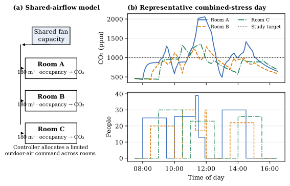
Three well-mixed rooms draw from one limited fan command. The representative day shows why allocation matters: an unannounced room change creates a local CO₂ peak while scheduled and actual occupancy disagree. Line style and colour both distinguish rooms; all figure text is black.
The second disturbance is mechanical rather than behavioural. Between 10:45 and 13:45, total available command falls from 2.05 to 1.35. No controller can give every room its preferred airflow during that interval. It must allocate scarcity.
A small mass balance with visible assumptions
The room model is intentionally simple. For room (i), the CO₂ state evolves as
Here (C_o=430) ppm is outdoor concentration, (V=180) m³ is room volume, (G=0.0045) L s⁻¹ person⁻¹ is the assumed occupant generation rate, and (N_{i,k}) is actual occupancy. The air-change rate depends on command (u_{i,k}):
The rooms are coupled only through capacity:
This is a well-mixed tracer model. It assumes a single concentration represents the whole room. It does not resolve supply jets, doors, leakage paths, recirculation, filters, or where a wall sensor sits. Occupant generation is constant within a time step even though metabolism varies between people and activities.
Those omissions define what the experiment can say. It can compare algorithms under a controlled mass balance. It cannot specify a real school’s ventilation rate.
The 1000 ppm line needs the same care. Persily and de Jonge explain that the familiar value emerged from a ventilation-rate and CO₂-generation relationship, not a direct health-effect threshold. In this project it is only a study target: a consistent line for measuring occupied exposure. “Above target” does not mean “unsafe,” and “below target” does not prove adequate indoor air quality.
Four ways to allocate air
The comparison uses four controllers.
- Fixed schedule maps the published headcount directly to airflow. It starts early enough to use timetable information but cannot react to an unrecorded room move.
- Reactive CO₂ raises command as measured concentration climbs. It responds to surprises but only after the tracer has accumulated.
- Schedule MPC predicts six five-minute steps using the timetable and searches a small set of feasible command triples.
- Buffered MPC runs the same search after adding five students to every forecast active room and using a more conservative internal control target.
The predictive objective combines occupied concentration exceedance, cubic fan effort, and changes in command:
This is not an industrial MPC implementation. The command remains constant over the short forecast during each candidate evaluation, the levels are discrete, and the buffer is a fixed headcount rather than a calibrated probability bound. The simplicity is useful because every decision can be reproduced and criticised.
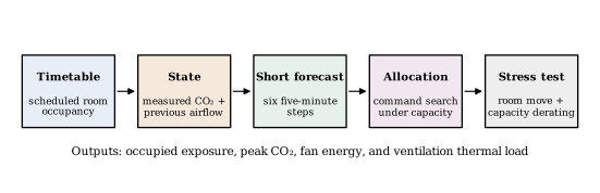
The timetable supplies a forecast, measured CO₂ supplies the current state, and the allocator must respect the shared command limit. Room changes and capacity derating are introduced only for evaluation.
A matched experiment, not four different lucky days
Each of the four conditions contains 120 replicates per controller:
| Condition | Timetable mismatch | Shared-capacity loss |
|---|---|---|
| Nominal | No | No |
| Room change | Yes | No |
| Capacity derating | No | Yes |
| Combined stress | Yes | Yes |
Within a condition and replicate, every controller sees the same attendance factors, room-change event, outdoor-temperature path, and capacity profile. This matching matters. If buffered MPC received easier random days, a difference in average exposure would say little about the controller.
The primary metric is occupied person-weighted exposure:
A five-minute interval with 30 people therefore counts more than an interval with three. Empty-room exceedance does not enter this primary measure. Secondary outputs include occupied mean CO₂, the unweighted whole-day maximum, fan energy, and outdoor-air thermal load. All energy quantities are model proxies rather than meter readings.
Means receive bootstrap 95% intervals. The direct buffered-minus-schedule comparison uses paired bootstrap resampling, preserving the common random day.
What changed under stress
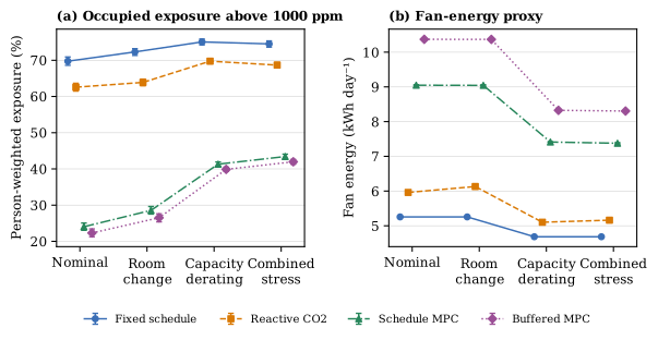
Mean occupied exposure and fan-energy proxy across four conditions. Each point uses 120 matched synthetic days; error bars are bootstrap 95% intervals. Markers and line styles make the comparison independent of colour.
The combined-stress averages are:
| Controller | Exposure above 1000 ppm | Fan proxy | Occupied mean CO₂ | Whole-day peak |
|---|---|---|---|---|
| Fixed schedule | 74.5% | 4.69 kWh/day | 1057 ppm | 1439 ppm |
| Reactive CO₂ | 68.7% | 5.16 kWh/day | 1036 ppm | 1417 ppm |
| Schedule MPC | 43.4% | 7.38 kWh/day | 1028 ppm | 1846 ppm |
| Buffered MPC | 42.0% | 8.30 kWh/day | 1026 ppm | 1854 ppm |
Two conclusions are well supported inside the generator.
First, looking ahead changes the allocation substantially. The predictive controllers spend more fan effort and reduce occupied exceedance by about 25–33 percentage points relative to the two simple baselines under combined stress. This is not a free efficiency gain. It is a different operating point with higher airflow cost.
Second, the additional forecast buffer has a much smaller effect. Against schedule MPC on identical days, the five-student buffer changes exposure by -1.45 percentage points. The paired 95% interval is -1.71 to -1.21 points. Fan energy changes by +0.93 kWh/day, with an interval of +0.91 to +0.94.
The correct reading is not that five is an optimal buffer. It is that this particular margin buys a measurable but modest change at a visible cost.
Why the worst peak moves in the wrong direction
The whole-day peak exposes a conflict hidden by the primary metric. Schedule MPC averages 1846 ppm under combined stress; buffered MPC averages 1854 ppm. The paired increase is 7.9 ppm, with a 95% interval from 1.1 to 14.6.
Why can a more conservative controller produce a larger maximum?
The objective protects forecast occupied person-time. When capacity binds, it can direct more air toward rooms expected to contain students. An unannounced transfer creates occupancy where the timetable predicts less. That room can be deprioritised while another scheduled room receives the buffer. The person-weighted total improves slightly, but the single worst room-time value becomes worse.
This is not a coding footnote. It is a decision question. Is the building trying to minimise total occupied exposure, prevent any room crossing a hard ceiling, protect the worst-served class, or balance these goals? A controller can only optimise the objective it is given.
The price of adding more margin
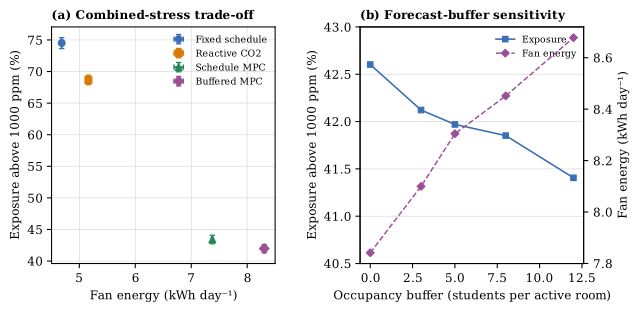
Left: combined-stress exposure versus fan energy. Right: the sensitivity of buffered MPC as the assumed extra headcount rises from zero to 12 students per active room. The right exposure axis is deliberately narrow because the effect is small.
The buffer sweep makes diminishing returns visible:
| Added forecast students | Exposure above 1000 ppm | Fan proxy |
|---|---|---|
| 0 | 42.6% | 7.84 kWh/day |
| 3 | 42.1% | 8.10 kWh/day |
| 5 | 42.0% | 8.30 kWh/day |
| 8 | 41.9% | 8.45 kWh/day |
| 12 | 41.4% | 8.68 kWh/day |
Increasing the margin from zero to 12 students changes exposure by only 1.2 percentage points while increasing fan energy by 0.84 kWh/day. The curve does not reveal a universal optimum. Change the fan model, command grid, climate, timetable, room volume, or cost weights, and the preferred point can move.
What this experiment leaves unresolved
Four boundaries should travel with the result.
The air is perfectly mixed
Real concentration varies across a room. A sensor near a return grille may not represent the breathing zone, and door opening can create exchanges not represented by a single air-change rate.
CO₂ is not the whole of indoor air quality
The model contains no particles, volatile compounds, filtration, aerosol source, or infection process. It cannot translate lower modelled CO₂ exposure into a quantified health outcome.
Energy is only a proxy
The fan term follows a cubic command relationship and the thermal-load term uses outdoor-air conditioning demand. There is no commissioned fan curve, chiller or heat-pump efficiency map, tariff, humidity process, or measured building load.
The controller has not seen a school
Every result comes from the project’s own generator. The same code defines attendance uncertainty, room changes, capacity loss, and the controller model. A field test must calibrate on one period or building and evaluate on independently recorded days without tuning against the answer.
Reproduction and editorial control
The ScienceProject directory contains the configuration, controller source, four unit tests, all 1,920 controller-condition trial rows, aggregate metrics, paired contrasts, buffer sweep, claim-evidence map, source ledger, technical study, and generating code for the four SVG figures.
Only files in figures/publish/ enter the public asset synchronisation process. Trial CSV files, caches, QA images, technical notes, and source code remain in ScienceProject. This article is manually written; rerunning the experiment can update the evidence and approved figures but cannot overwrite the interpretation.
That separation is important here. A metric table can say the buffer reduced exposure by 1.45 points. It cannot decide whether the extra 0.93 kWh/day, higher worst peak, and missing field evidence make that a sensible building policy.
Sources and intellectual lineage
Persily and de Jonge provide the occupant CO₂-generation and mass-balance context, including a warning against treating a familiar concentration value as a direct health threshold. Earlier NIST guidance on CO₂-based demand-controlled ventilation frames control in terms of actual or surrogate occupancy and identifies sensor and operational concerns.
The FRESH classroom intervention supplies field evidence that controlled ventilation can change measured classroom CO₂. Petersen and colleagues studied increased classroom ventilation and schoolwork performance in a crossover intervention. A recent field implementation of occupancy-aware predictive control in a school building shows that this control family is being tested in real institutional buildings.
These studies motivate the question and model lineage. None validates the numerical values reported here; those come only from this synthetic benchmark.
Conclusion
A timetable is valuable because it lets ventilation act before CO₂ rises. It is dangerous when the controller treats prediction as truth.
In this benchmark, short-horizon allocation materially reduces person-weighted exposure relative to fixed and reactive baselines, but uses more fan command. Adding a simple occupancy buffer improves the primary metric only slightly, costs additional energy, and worsens the whole-day maximum. The next useful experiment is therefore not a larger claim. It is an instrumented classroom study where the model, fan law, timetable errors, and evaluation days are measured independently.