When Treatment Spills Over

Treat one person, classroom, neighbourhood, or seller, and someone else may change.

That possibility is not an inconvenience at the edge of causal inference. In many social, educational, epidemiological, and marketplace interventions, it is part of the mechanism. Information is shared, infections are prevented, queues are displaced, and behaviours are imitated. The outcome of unit $i$ may depend on the treatment assigned to unit $j$ .

The usual difference between treated and untreated outcomes becomes difficult to interpret in this setting. Treated units may also have more treated neighbours. Untreated units may receive indirect exposure. Two random assignments with the same treatment coverage can produce different contrasts because they place treatments differently on the network.

The network-interference laboratory exposes this problem with a small synthetic graph. The lesson is not that one particular estimator is always biased. It is that the treatment effect must be defined together with the interference structure and the assignment design.

Potential outcomes depend on an assignment vector

Without interference, a potential outcome is often written $Y_i(z_i)$ : the outcome unit $i$ would show under its own treatment $z_i$ . With interference, the potential outcome can depend on the full assignment vector,

Y_i(\mathbf z)=Y_i(z_1,z_2,\ldots,z_n).

This formulation is general but impossible to estimate without further structure. For $n$ binary treatments, each unit could in principle have $2^n$ potential outcomes. A single experiment reveals only one assignment vector.

An exposure mapping reduces that space by asserting which features of the assignment matter for each unit. In the interactive model,

E_i(\mathbf z)=\frac{1}{|\mathcal N(i)|}\sum_{j\in\mathcal N(i)}z_j

is the treated fraction of $i$ ‘s neighbours, and the synthetic outcome is

Y_i=\alpha_i+\tau z_i+\gamma E_i.

Here $\tau$ is a direct effect at fixed neighbour exposure and $\gamma$ controls spillover. The model is intentionally transparent: the network, exposure rule, and coefficients are known. A real study does not receive those elements for free.

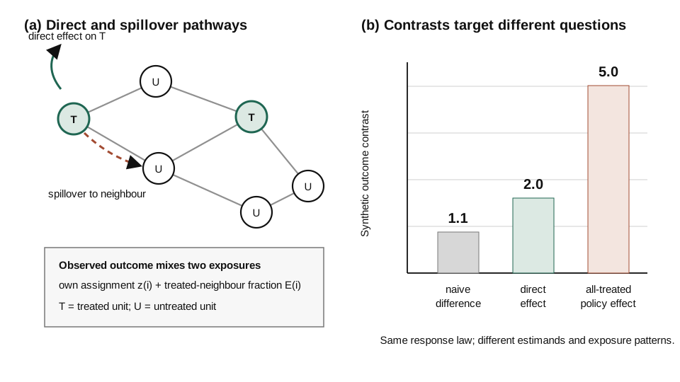
Two-panel schematic showing treatment and spillover paths on a network and a comparison of naive, direct, and policy-effect contrasts. — **Figure 1.** Interference changes both the data structure and the question being answered. Panel (a) separates a unit's own treatment from exposure transmitted by treated neighbours. Panel (b) uses a synthetic example to show that a naive treated-minus-untreated difference, a direct effect, and an all-treated policy effect are distinct quantities.

The network view explains why the naive contrast can move even when the direct response coefficient is fixed. Treated and untreated groups can inherit different neighbour-exposure distributions, so their observed difference mixes receipt, spillover, and assignment pattern.

Aronow and Samii organise general interference around three connected choices: the randomisation design, the mapping from assignments to exposures, and the estimand. That triad is a useful discipline. It prevents the analyst from choosing an exposure definition only after seeing which one produces the desired result.

One phrase, several causal questions

“The treatment effect” can refer to different contrasts under interference.

A direct effect compares a unit treated and untreated while holding its surrounding exposure fixed. A spillover effect compares two neighbour-exposure conditions for a unit whose own treatment is fixed. A total or policy effect compares two assignment regimes, such as treating everyone versus treating no one.

These are not interchangeable. In the laboratory, the direct coefficient is $\tau=2$ . The all-treated versus none-treated policy contrast is $\tau+\gamma$ because every unit changes both its own treatment status and its neighbour exposure. The naive treated-minus-untreated difference is neither quantity in general. It also contains differences in average exposure and in the small heterogeneous baselines used by the simulation.

Move the assignment-pattern control while keeping treatment coverage and $\gamma$ fixed. The direct and all-treated policy effects remain unchanged by construction, but the naive contrast moves. That movement is a design effect, not a change in the underlying response law.

This is why a causal paper should name the estimand in operational language. “Effect of the programme” is incomplete if readers cannot tell whether it means receipt, indirect exposure, saturation, or a change in the treatment policy.

The graph is part of the measurement system

Network interference requires a defensible account of who can affect whom. Friendship nominations, geographic proximity, classroom membership, shared infrastructure, buyer–seller interactions, or communication records generate different graphs. Each captures some pathways and misses others.

Measurement error in the graph can misclassify exposure even when treatment assignment is perfectly recorded. Missing edges can label an indirectly exposed unit as unexposed. Time aggregation can place an interaction before or after treatment incorrectly. A network observed after the intervention may itself have changed because of treatment.

The graph should therefore be treated as data with provenance, uncertainty, and temporal scope. Sensitivity analysis can repeat the estimation under plausible alternative neighbourhoods. Negative-control pathways can test whether effects appear along edges that should not transmit the intervention. When the graph is too uncertain, clustered or geographic exposure categories may be more defensible than a highly detailed but fragile network score.

Design determines which exposures are observable

Randomisation does not automatically solve interference. A design that almost never produces isolated treated units cannot estimate an effect for that exposure condition with useful precision. This is a positivity problem: the assignments required to define the contrast must occur with nonzero and sufficiently large probability.

Cluster randomisation can increase the probability of high and low neighbour exposure, making policy-like contrasts easier to estimate. It can also make direct effects at fixed exposure difficult because treatment and local exposure move together. Individual randomisation provides different exposure variation but may generate substantial mixing between conditions.

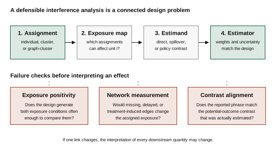
Workflow linking assignment design, exposure mapping, causal estimand, and estimator, with checks for positivity, network measurement, and contrast alignment. — **Figure 2.** A defensible interference study is a connected design problem. The assignment must generate the exposures used by the estimand, and the estimator must respect their assignment probabilities. Positivity, network measurement, and contrast alignment are failure checks rather than afterthoughts.

This sequence is directional. If the exposure map changes after discovering missing edges, the relevant estimand and weighting scheme may also change. A valid randomisation procedure cannot rescue an effect label that no longer matches the measured exposure.

In two-sided systems, the treated and measured units may not even be the same population. A marketplace may randomise sellers while measuring buyer outcomes; an advertising system may change campaigns while measuring users. Harshaw and colleagues study such bipartite experiments under a linear exposure-response model and develop an exposure-reweighted estimator together with a design intended to improve precision. Their result illustrates a broader point: analysis and assignment should be designed together around the exposure variation needed by the estimand.

A concrete research pathway

The browser model can be extended into a serious simulation study without pretending that the synthetic graph is empirical evidence.

First, define two or three plausible exposure mappings for a target context: treated-neighbour fraction, distance-weighted exposure, and group saturation, for example. Second, compare individual, cluster, and graph-cluster assignment designs. Third, generate outcomes under mechanisms that deliberately violate each exposure mapping. Fourth, evaluate bias, interval coverage, and effective sample size for the direct, spillover, and policy estimands.

The central research question could be:

How sensitive are interference-aware estimators to plausible misspecification of the exposure network under assignment designs with equal treatment budgets?

That question is academically useful because many methodological guarantees assume the exposure mapping is known. A simulation can identify which combinations of design and estimator fail gracefully when edges are missing, spillover decays with distance, or the response is nonlinear. A later empirical study can then use those results to preregister the estimand and sensitivity analysis.

Another direction is adaptive policy. If interventions are rolled out sequentially, past outcomes may influence future assignments. Interference then interacts with time, feedback, and changing networks. The simple static mapping is no longer enough, but it provides the baseline that a dynamic model must improve upon.

What the interaction leaves unresolved

The laboratory assumes a fixed undirected graph, linear additive response, no hidden confounding, known treatment assignment, immediate exposure, and no measurement error. It does not calculate an inverse-probability estimator or a randomisation-based variance. The displayed naive contrast comes from one deterministic synthetic assignment rather than repeated randomisation.

The model also assumes that the treated-neighbour fraction is sufficient. Two units with the same fraction but very different neighbours receive the same exposure. Thresholds, repeated contact, direction, timing, tie strength, and higher-order groups are omitted.

These omissions make the model teachable. They also define the boundary of the claim. The interaction shows how estimands diverge under one transparent interference mechanism; it does not identify spillovers in any real network.

Conclusion

Interference does more than add correlation between observations. It changes which potential outcomes exist and which causal contrasts are meaningful.

A defensible analysis therefore begins before estimation. It specifies who can affect whom, maps assignments to exposures, chooses a design that produces those exposures, and names the direct, spillover, or policy contrast the study intends to learn.

When treatment spills over, the graph is not merely a visualisation. It is part of the causal question.

References

Hudgens, M. G., & Halloran, M. E. (2008). Toward causal inference with interference. Journal of the American Statistical Association, 103(482), 832–842. https://doi.org/10.1198/016214508000000292
Aronow, P. M., & Samii, C. (2017). Estimating average causal effects under general interference, with application to a social network experiment. The Annals of Applied Statistics, 11(4), 1912–1947. https://doi.org/10.1214/16-AOAS1005
Harshaw, C., Sävje, F., Eisenstat, D., Mirrokni, V., & Pouget-Abadie, J. (2023). Design and analysis of bipartite experiments under a linear exposure-response model. Electronic Journal of Statistics, 17(1), 464–518. https://doi.org/10.1214/23-EJS2111
Ogburn, E. L., & VanderWeele, T. J. (2014). Causal diagrams for interference. Statistical Science, 29(4), 559–578. https://doi.org/10.1214/14-STS501