Natural selection is directional, but evolution in a finite population is not deterministic.
A new allele can increase expected reproductive success and still disappear in its first few generations. A locally favourable allele can be held at low frequency by migration. A population can recover numerically after a bottleneck while remaining genetically depleted. These outcomes are not exceptions added to an otherwise deterministic theory. They follow from sampling.
This study uses a diploid Wright–Fisher model to connect four ideas—drift, selection, migration, and bottlenecks—inside one reproducible synthetic experiment. The purpose is not to infer the history of a real population. It is to show which qualitative claims survive explicit simulation and which require empirical data.
The model starts with copies, not percentages
Consider a diploid population of size (N). If allele (A) has frequency (p_t), there are (2N p_t) copies before reproduction. With genic selection coefficient (s), the expected frequency after selection is
The next generation is sampled rather than assigned:
The binomial step is the source of drift. Its conditional variance,
shrinks as (N) grows, but it never vanishes in a finite population. The states (p=0) and (p=1) are absorbing when mutation and migration are absent. A trajectory eventually loses or fixes the allele.
That formulation also clarifies why “a beneficial mutation has selection coefficient (0.05)” is incomplete. Starting frequency matters. In this experiment every fixation run begins from one copy,
Larger populations reduce drift per generation, but they also make a single copy a smaller initial fraction of the population.
Selection changes odds, not destiny
The fixation grid used five population sizes and six selection coefficients, with 2,500 independent replicates for every parameter pair. Under neutrality, the fixation probability of one copy should equal (1/(2N)). The simulation recovered that benchmark closely: (0.0248) for (N=20), (0.0056) for (N=100), and (0.0008) for (N=500), compared with theoretical values (0.025), (0.005), and (0.001).
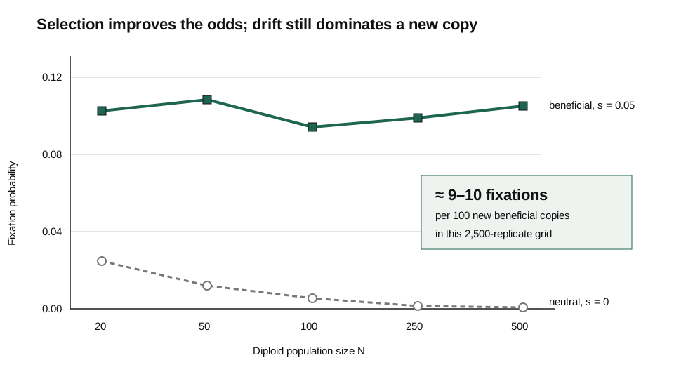
At (s=0.05), fixation increased to (0.0952), (0.1016), (0.0868), (0.0924), and (0.0992) as (N) ranged from 20 to 500. The approximate constancy is consistent with the strong-selection, rare-copy regime: selection offsets the declining initial frequency, but it does not make fixation likely.
The practical lesson is sharper than “small populations have more drift.” A beneficial allele introduced once has a high probability of early loss even when its expected trajectory points upward. Reporting only the deterministic recurrence hides the event that dominates most realizations.
Migration can oppose local adaptation
The model extends to two demes by applying migration before selection and sampling. If (m) is the symmetric migration fraction,
Selection then acts with opposite signs in the two habitats. The experiment therefore asks whether a locally favoured allele can remain differentiated when migrants continually import the alternative.
This is not a contest between a universally “good” allele and random noise. Fitness is environment-specific. Weak migration can replenish variation and reduce local loss; stronger migration can homogenize the demes and erode the response to divergent selection. The relevant dimensionless comparison is not (m) or (s) alone, but their scale relative to drift and to one another.
The synthetic results support a trade-off, not a universal migration threshold. An empirical application would require defensible effective population sizes, direction-specific migration, dominance, linked loci, and an observation model for sampled genotypes.
A bottleneck is remembered after abundance recovers
Expected heterozygosity,
measures within-locus diversity. Under neutral Wright–Fisher drift,
The simulation checked this decay law using 8,000 independent loci per population size. It then imposed a ten-generation bottleneck from (N=500) to (N_b), after which census size returned immediately to 500.
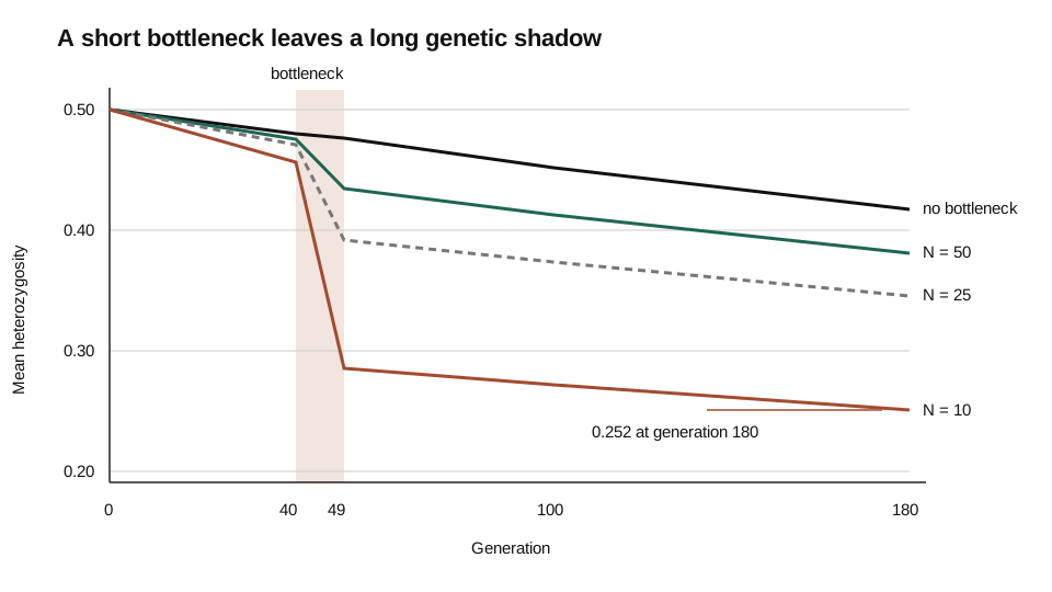
At generation 180, mean heterozygosity was approximately (0.417) without a bottleneck and (0.252) after a bottleneck to (N_b=10). Intermediate bottlenecks ended at (0.345) for (N_b=25) and (0.381) for (N_b=50).
This is a useful separation of state variables. Census size can rebound in one generation because the model instructs it to do so. Allele-frequency diversity cannot rebound without mutation, migration, or stored variation. Demographic recovery and genetic recovery are different claims.
What the computation validates
The supplied run completed a five-by-six fixation grid, neutral diversity checks, migration experiments, and bottleneck experiments. It used 2,500 fixation replicates per cell, 8,000 loci for the neutral validation, 1,800 replicates per migration setting, and 10,000 loci per bottleneck scenario. Six unit tests and the output-manifest checks passed.
Those checks support the implementation of the stated model. They do not validate the model for a particular species. The experiment omits mutation, dominance, overlapping generations, linkage, changing population size outside the bottleneck, and uncertainty in (N_e). It also treats loci as independent.
The next research step is therefore not simply a larger simulation. A stronger study would add an observation layer and ask which combinations of (N_e), (s), and (m) are identifiable from finite time-series or genomic samples. It could then compare conservation policies under posterior uncertainty rather than under known parameters.
Conclusion
Selection supplies a direction; drift supplies a distribution of possible histories. Migration couples those histories across space, and bottlenecks remove options that later demographic growth cannot automatically recreate.
The model’s most important result is not a single fixation probability. It is a discipline for interpretation: distinguish expected change from realized trajectories, abundance from diversity, and model validation from empirical validation.
References
- Wright, S. (1931). Evolution in Mendelian populations. Genetics, 16(2), 97–159. https://doi.org/10.1093/genetics/16.2.97
- Kimura, M. (1962). On the probability of fixation of mutant genes in a population. Genetics, 47(6), 713–719. https://doi.org/10.1093/genetics/47.6.713
- Shafiey, H., & Waxman, D. (2017). Exact results for the probability and stochastic dynamics of fixation in the Wright–Fisher model. Journal of Theoretical Biology, 430, 64–77. https://doi.org/10.1016/j.jtbi.2017.06.026
- Whitlock, M. C. (2003). Fixation probability and time in subdivided populations. Genetics, 164(2), 767–779. https://doi.org/10.1093/genetics/164.2.767
- Nei, M., Maruyama, T., & Chakraborty, R. (1975). The bottleneck effect and genetic variability in populations. Evolution, 29(1), 1–10. https://doi.org/10.1111/j.1558-5646.1975.tb00807.x