Can One Local Pulse Stop a Travelling Excitation Wave?

An excitable medium can rest quietly until a sufficiently large disturbance creates a travelling pulse. Behind the front, a slower recovery variable temporarily prevents immediate re-excitation. This activator–recovery architecture appears in models of nerve impulses, chemical reactions, ecological waves, and cardiac tissue, although the interpretation and parameters differ greatly.

The control question here is deliberately generic:

Can a small number of local, event-triggered interventions stop a travelling excitation wave robustly under uncertain conduction speed and sensor delay?

The study is not a medical treatment proposal. It uses a one-dimensional FitzHugh–Nagumo-type model as a controlled benchmark for sparse spatiotemporal control.

The model and control geometry

Let $u(x,t)$ be a fast activator and $v(x,t)$ a slow recovery field:

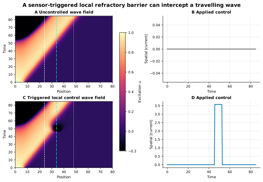
\frac{\partial u}{\partial t} =D\frac{\partial^2u}{\partial x^2} +u(u-a)(1-u)-v+I(x,t),

\frac{\partial v}{\partial t} =\varepsilon(u-\gamma v).

A localized initial disturbance launches a pulse. A sensor at $x_s=24$ detects the wave. After a communication delay, an actuator centered at $x_a=34$ applies a negative current over width 5 for a chosen amplitude and duration. A downstream monitor at $x_m=48$ decides whether the wave passed.

This separation prevents a trivial solution. The actuator cannot act before upstream evidence arrives, and the monitor lies far enough downstream that an uncontrolled wave normally has time to reach it.

Space-time activation field showing sensor trigger, localized intervention, wave attenuation and downstream monitor. — **Figure 1.** Representative control story. The sensor, delayed trigger, actuator footprint, and downstream monitor are all visible, making the causal timing inspectable.

A false success found during development

An early configuration reported near-perfect “blocking” even with no control. The wave either decayed before reaching the monitor or the simulation ended too early. That was not a successful controller; it was a defective evaluation geometry.

The repair changed recovery parameters, monitor position, and travel-time logic so an ordinary uncontrolled wave reaches the monitor in most held-out cases. The final no-control success rate is $0.233$ , not one. This episode is methodologically important. A benchmark can be easy for the wrong reason, and a high score does not diagnose that error.

Three checks should accompany any wave-blocking benchmark:

an uncontrolled positive control must propagate in the intended regime;
a strong global intervention should demonstrate that blocking is dynamically possible;
the time horizon must exceed a conservative travel-time estimate.

Training the local policy

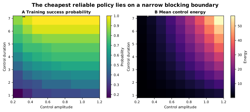
The candidate policy grid varies negative-current amplitude and duration. For each pair, simulations cover uncertain diffusion, recovery rate, and sensor delay. The objective favours high blocking probability and low integrated squared current,

E=\int_0^{t_f}\int_0^L I(x,t)^2\,dx\,dt.

The selected local policy uses amplitude $0.325$ and duration $7.2$ . On the training ensemble it blocks $95.24\%$ of waves with mean energy $4.183$ .

Policy map of local intervention amplitude and duration with blocking probability and energy. — **Figure 2.** Amplitude–duration policy map. A broad high-success region exists, but energy rises with stronger and longer forcing; the chosen policy is a compromise rather than the most forceful point.

Frozen held-out comparison

After selection, amplitude and duration are frozen. Thirty-six unseen combinations of diffusion, recovery rate, and delay are evaluated.

No control: success $0.233$ , energy $0$ .
Periodic global forcing: success $1.000$ , energy $29.428$ .
Triggered local forcing: success $0.944$ , energy $4.183$ .

The local policy therefore uses about one seventh of the global baseline energy while losing roughly 5.6 percentage points of blocking probability.

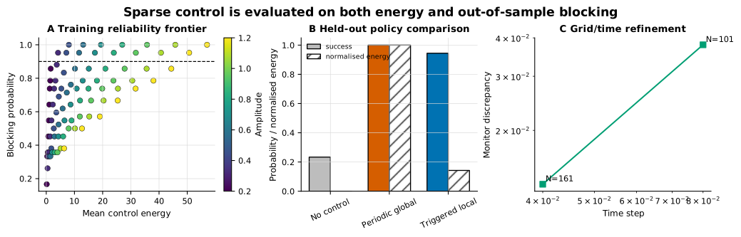
Held-out blocking probability versus intervention energy for no control, periodic global and triggered local policies. — **Figure 3.** Held-out success–energy frontier. Global forcing is more reliable in this benchmark but far more expensive; local control occupies a distinct compromise.

This is a multi-objective result. If one failed passage is unacceptable and energy is cheap, global forcing is preferable inside the simulator. If energy or intervention area matters, the local policy is attractive. The mathematics does not choose how to value those outcomes.

What “blocked” means

Blocking is defined by the maximum downstream activator remaining below a threshold after enough travel time. This operational definition can fail in two ways:

a delayed weak pulse might cross after the observation window;
a harmless subthreshold remnant can still count as failure if the line is set too low.

The study therefore reports the mean monitor peak beside binary success and uses a travel-time forecast to set the horizon. A stronger future analysis would estimate wave-front position continuously and distinguish extinction, reflection, delay, and fragmentation.

The representative policy is rerun at grids 101, 161, and 241 with time steps $0.08$ , $0.04$ , and $0.025$ . All three classify the case as blocked. Monitor peaks approach the fine value: the difference falls from $0.0380$ to $0.0134$ and then zero by reference definition.

Energy varies from $3.65$ to $4.21$ and $3.82$ because the rectangular actuator is represented on different discrete grids. This is not hidden. For stronger convergence, the actuator footprint should be integrated with grid-independent quadrature or smoothed spatially.

Mechanistic interpretation

The negative pulse acts ahead of the incoming wave and temporarily reduces excitability. Successful timing creates a region in which the activator front cannot sustain itself while the recovery field remains inhibitory. Too weak or short an action leaves enough activator to recover. Excessively delayed action arrives after the front has crossed the actuator.

The model also shows why event-triggering can outperform periodic sparse timing: the sensor aligns intervention with realized wave arrival. But sensor delay uncertainty sets a hard limit. If delay is long relative to the sensor–actuator travel time, no amplitude selected under the current safety bounds can restore causality.

Claim boundary

The supported statement is:

In the declared one-dimensional excitable-medium benchmark, a frozen local policy with amplitude $0.325$ and duration $7.2$ blocks $94.44\%$ of held-out waves using energy $4.183$ , compared with $100\%$ and energy $29.428$ for periodic global forcing.

It does not imply cardiac, neurological, or chemical-process safety. The FitzHugh–Nagumo variables are generic; the geometry is one-dimensional; uncertainty ranges are synthetic; tissue anisotropy, three-dimensional scroll waves, refractory heterogeneity, measurement artefacts, and hardware limits are absent.

References

R. FitzHugh, “Impulses and physiological states in theoretical models of nerve membrane,” Biophysical Journal, 1961. doi:10.1016/S0006-3495(61)86902-6.
J. Nagumo, S. Arimoto, and S. Yoshizawa, “An active pulse transmission line simulating nerve axon,” Proceedings of the IRE, 1962. doi:10.1109/JRPROC.1962.288235.
J. Siehr et al., “Targeting characteristic wave properties in reaction-diffusion systems by optimization of external forcing,” Physical Review E, 2007. doi:10.1103/PhysRevE.76.056211.
E. A. Ermakova et al., “On propagation of excitation waves in moving media: the FitzHugh–Nagumo model,” PLoS ONE, 2009. doi:10.1371/journal.pone.0004454.