Ask the Oscillator the Experiment That Separates Its Models

Collecting more data is not the same as collecting discriminating data. Two nonlinear models can produce similar free oscillations yet respond very differently to a carefully chosen forcing frequency and amplitude. If only a handful of experiments are available, the next input should be selected for what it can reveal.

This benchmark asks:

Which forcing amplitudes and frequencies most efficiently distinguish competing nonlinear oscillator mechanisms under a limited experiment budget?

Three candidate families compete: Van der Pol, Rayleigh, and Duffing. The problem is closed-world and synthetic; posterior probabilities are conditional on these families and their parameter priors.

Competing mechanisms

Representative forms are

\ddot x-\mu(1-x^2)\dot x+x=A\cos(\omega t)

for Van der Pol,

\ddot x+\mu(\dot x^2-1)\dot x+x=A\cos(\omega t)

for Rayleigh, and

\ddot x+\delta\dot x+\alpha x+\beta x^3=A\cos(\omega t)

for Duffing.

All can sustain or reshape oscillations, but nonlinear damping and nonlinear stiffness respond differently to forcing. Each model carries 26 parameter particles. An experiment applies one amplitude–frequency pair and observes a compressed late-time response with Gaussian noise $0.65$ .

Predictive-separation landscape over forcing amplitude and frequency for three nonlinear oscillator models. — **Figure 1.** Design landscape. Informative forcing lies where model predictive distributions separate, not necessarily where the response amplitude is largest.

Sequential Bayesian update

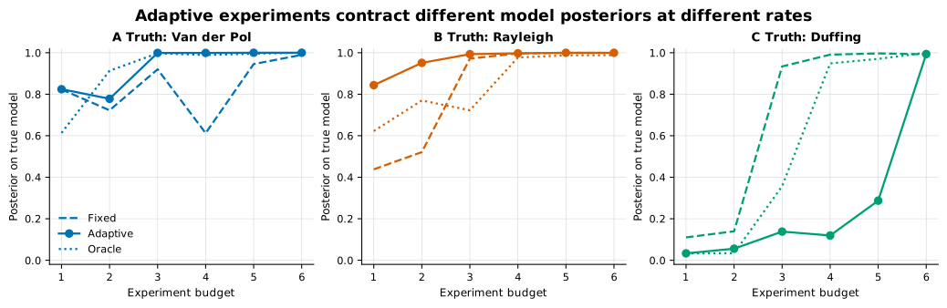
Before each round, model and parameter particles define predictive distributions for every unused candidate experiment. The adaptive score rewards robust between-model separation relative to within-model parameter variation and observation noise.

The highest-scoring unused forcing is applied. Bayes’ rule updates particle and model weights:

p(M,\theta\mid z,d)\propto p(z\mid M,\theta,d)p(\theta\mid M)p(M),

where $d$ is the design and $z$ the compressed observation. The process repeats for six rounds.

The fixed baseline follows a space-filling schedule independent of observations. An oracle knows the true model family but not its parameter; it provides an upper comparison and is not deployable.

Why the benchmark was made harder

An initial version was too easy: long, low-noise trajectories made all strategies nearly perfect. That ceiling would not test adaptive design. The final benchmark compresses observations and raises noise to $0.65$ , creating overlap among predictive distributions while retaining identifiable regions.

This change illustrates an important principle. Difficulty should come from the intended inference problem, not from bugs or missing information. The benchmark remains solvable by a good design, but a generic schedule has measurable uncertainty.

Final performance

Across 70 trials for each true model:

Adaptive: accuracy $1.000$ , mean true-model probability $0.992$ , Brier score $0.00287$ .
Fixed: accuracy $0.9619$ , mean true-model probability $0.952$ , Brier score $0.0509$ .
Oracle: accuracy $1.000$ , mean true-model probability $0.995$ , Brier score $0.00172$ .

Posterior model probabilities over six sequential experiments for adaptive and fixed strategies. — **Figure 2.** Posterior paths. Adaptive design often creates a decisive separation in fewer rounds; fixed experiments can spend budget where all models predict similar summaries.

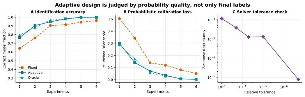
Accuracy alone would understate the difference because both methods are strong. The Brier score measures probabilistic calibration and sharpness. The fixed strategy’s occasional ambiguity remains visible even when its final top-1 label is correct.

Accuracy, true-model probability and Brier score for adaptive, fixed and oracle experimental design. — **Figure 3.** Accuracy and calibration. The adaptive method closes most of the gap to the oracle within the declared candidate set.

What the design score is really doing

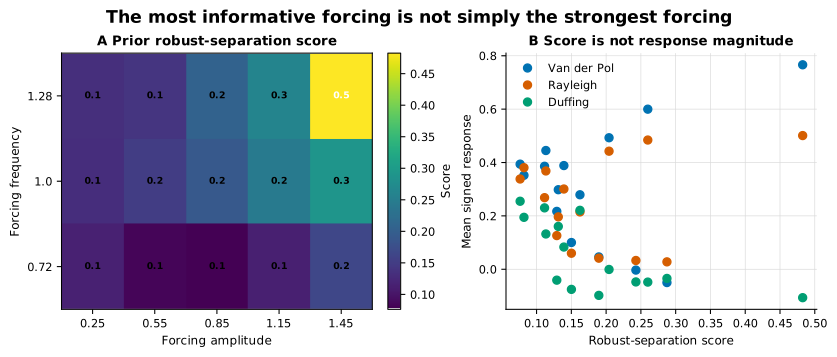
A forcing is informative when different models make separated predictions after integrating over parameter uncertainty. Large output is not enough. If all three families resonate similarly, a dramatic trajectory can be nearly useless for discrimination.

The score also avoids experiments whose apparent separation depends on a narrow particle. Robust separation requires different model clouds to be apart relative to their internal spread. This is the experimental-design analogue of comparing an effect size with uncertainty rather than ranking raw means.

Solver verification

Model discrimination can be corrupted if numerical integration error differs across model families or forcing regimes. Tightening tolerance from $10^{-3}$ to $2\times10^{-7}$ reduces the representative relative trajectory difference to $7.72\times10^{-8}$ . The non-monotone middle values around $10^{-5}$ are retained rather than hidden; adaptive solvers can change step sequences, so convergence need not be perfectly monotone at every tolerance.

The final reference error is far below observation noise. This supports interpreting posterior differences as model and data effects rather than integrator artefacts.

Closed-world posterior probabilities

A posterior of $0.992$ does not mean a 99.2% chance that nature uses the named equation. It means that, conditional on:

one of the three candidate families being true;
the stated parameter priors;
the observation summary and noise model;
the forcing candidate set;
and the numerical simulator,

the observed sequence strongly favours the generating family.

Real model discrimination needs an “all models wrong” route: posterior predictive checks, discrepancy models, expanded mechanisms, and experiments that can expose shared failure.

Claim boundary

The supported result is:

In the declared six-round synthetic benchmark, adaptive predictive-separation design reaches 100% classification accuracy and Brier $0.00287$ , compared with 96.19% and Brier $0.0509$ for a fixed space-filling schedule.

It does not identify a real oscillator. The advantage may change with candidate designs, priors, summaries, costs, or unmodeled dynamics.

References

A. C. Atkinson and A. N. Donev, Optimum Experimental Designs, Oxford University Press, 1992.
K. Chaloner and I. Verdinelli, “Bayesian experimental design: A review,” Statistical Science, 1995. doi:10.1214/ss/1177009939.
B. van der Pol, “On relaxation-oscillations,” The London, Edinburgh, and Dublin Philosophical Magazine, 1926. doi:10.1080/14786442608564127.
G. Duffing, Erzwungene Schwingungen bei veränderlicher Eigenfrequenz, 1918.