A No-Trade Band for Rough Volatility and Transaction Costs

Delta hedging suggests a simple instruction: update the stock position whenever option delta changes. In a frictionless Black–Scholes world with continuous trading, that instruction has a clean replication argument. Realized volatility is not constant, trading is discrete, and each rebalance costs money. Following every small delta movement can turn model responsiveness into unnecessary turnover.

This study asks:

Does a model-uncertainty-aware no-trade band reduce tail hedging loss when volatility roughness and transaction cost are misspecified?

It is a synthetic pricing-and-hedging experiment, not investment advice. The rough process is a controlled simulator rather than a calibrated market model.

Simulator and deliberately misspecified baseline

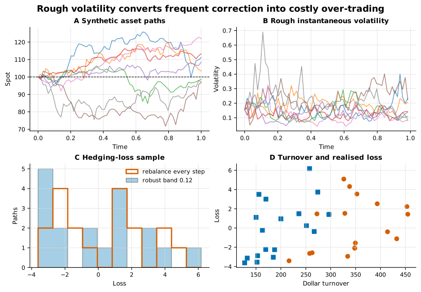
A correlated Gaussian convolution drives log variance with roughness parameter $H<1/2$ . The asset follows a geometric diffusion using the resulting stochastic variance. Importantly, the variance driver at each step uses only past and current available noise. An earlier implementation accidentally allowed same-step information to leak into the hedge; removing that look-ahead was necessary before interpreting any result.

The target hedge is Black–Scholes delta computed from a simple volatility estimate. That model is deliberately misspecified relative to the rough simulator. The full-delta policy moves to the target at every time step. A band policy trades only when the target leaves an interval of half-width $b$ around the current position.

Representative rough-volatility price, variance, delta and no-trade-band hedging paths. — **Figure 1.** Path-level mechanism. The band ignores small target movements and trades after a threshold crossing, so lower turnover is purchased with tracking error.

Select once, then freeze

Candidate bands are $0$ , $0.02$ , $0.05$ , $0.08$ , $0.12$ , and $0.18$ . Each is evaluated over a training grid of roughness, volatility-of-volatility, and transaction-cost scenarios. The objective minimizes the worst 95% conditional value at risk (CVaR) across training scenarios.

Band $0.12$ has the smallest training worst-case CVaR, approximately $8.738$ . The objective is non-monotone: $0.18$ trades less but worst-case CVaR rises to $9.256$ because tracking error dominates.

After selection, the band is frozen and evaluated on unseen intermediate and stress regimes. This separation is central. Choosing the best band independently in every test scenario would be an oracle comparison, not a deployable rule.

Held-out result

Across held-out regimes, selected-band mean CVaR is approximately $8.847$ , compared with $9.517$ for full delta. Mean turnover falls by $42.33\%$ .

Held-out stress map comparing tail hedging loss across roughness, volatility-of-volatility and costs. — **Figure 2.** Held-out stress map. The band is not re-tuned per cell; local losses reveal where the frozen decision succeeds and where it remains vulnerable.

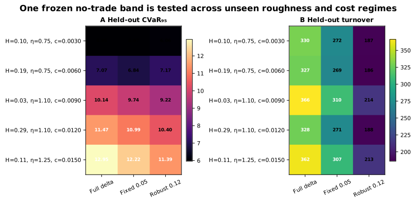
The claim is about the mean across declared held-out regimes. It does not imply that the band wins on every path or scenario. A band can lose when a rapid move makes delayed adjustment costly, and it can win when repeated small target changes would mostly generate fees.

Why CVaR and turnover are both needed

Mean hedging error can hide asymmetric tail loss. CVaR averages losses beyond a high quantile, focusing the objective on severe outcomes. Yet CVaR alone can favour a policy with excessive ordinary trading if costs are represented incompletely. Turnover supplies a second operational metric.

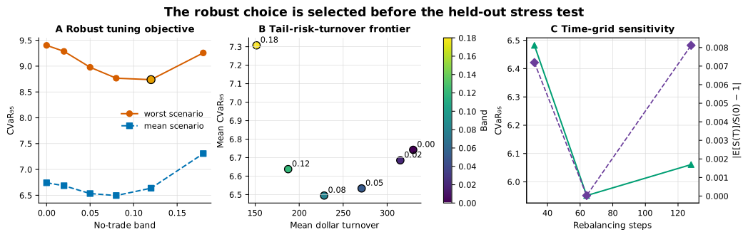
Frontier between held-out tail loss and turnover for candidate no-trade bands. — **Figure 3.** Tail-loss–turnover frontier. The selected $0.12$ band is a robust compromise inside this simulator, not a universal optimum.

The initial stock simulator also undergoes a martingale sanity check. Maximum absolute discounted-price error is approximately $0.00735$ over the tested configuration. This does not prove the discretized rough model is exact, but it would expose major drift or look-ahead errors.

What uncertainty robustness means

The training objective treats roughness, volatility-of-volatility, and cost as scenario dimensions. It does not estimate a posterior probability over them. “Robust” means the band is chosen to control the worst training CVaR and then tested without retuning.

Alternative robust formulations could produce different choices:

minimize average CVaR under scenario weights;
constrain turnover and minimize worst loss;
use distributionally robust neighborhoods;
optimize regret relative to a scenario oracle;
or adapt the band online from filtered state uncertainty.

The current formulation is useful because it is transparent and falsifiable.

Claim boundary

The supported statement is:

In the declared rough-volatility-inspired simulator, the frozen $0.12$ band reduces mean held-out CVaR from $9.517$ to $8.847$ and mean turnover by $42.33\%$ relative to full delta.

It does not establish expected profit, market calibration, arbitrage-free pricing accuracy, or live execution performance. It excludes order-book impact, discrete bid–ask dynamics, volatility-estimation error beyond the declared rule, jumps, funding, and model recalibration.

References

J. Gatheral, T. Jaisson, and M. Rosenbaum, “Volatility is rough,” Quantitative Finance, 2018. doi:10.1080/14697688.2017.1393551.
C. Bayer, P. Friz, and J. Gatheral, “Pricing under rough volatility,” Quantitative Finance, 2016. doi:10.1080/14697688.2015.1099717.
H. Buehler, L. Gonon, J. Teichmann, and B. Wood, “Deep hedging,” Quantitative Finance, 2019. doi:10.1080/14697688.2019.1571683.
P. Artzner et al., “Coherent measures of risk,” Mathematical Finance, 1999. doi:10.1111/1467-9965.00068.