Climbing Invisible Mountains: Heuristics on Fitness Landscapes

In the last post, we embraced “good enough.” This sequel goes deeper into the math of how heuristics move across rugged fitness landscapes—the invisible mountains where every coordinate encodes a solution and its height is the objective value. If you want a warm-up, skim the intro first:

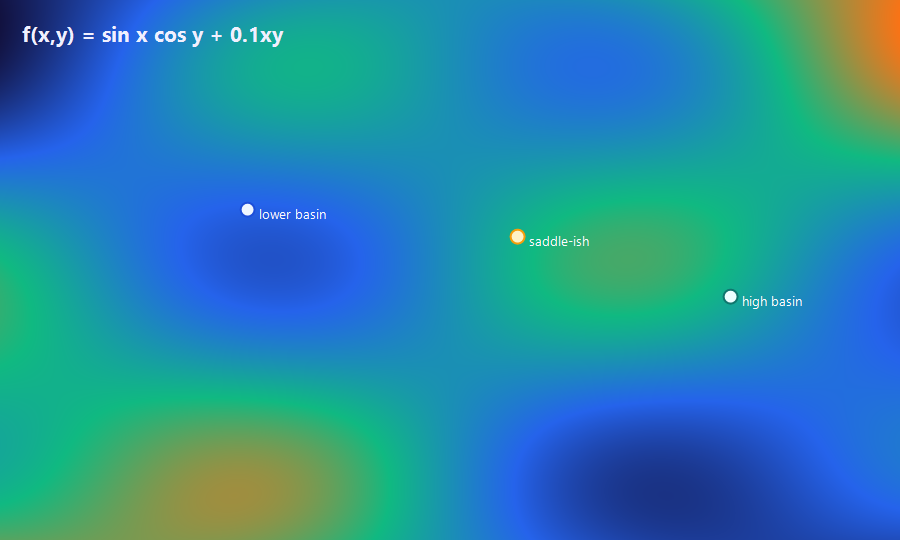Contour sketch with two basins and a saddle for $f(x,y) = \sin x \cos y + 0.1xy$.

A Landscape in One Equation

Suppose our objective is a noisy hill:

It has a tall peak near $(x \approx 2)$ and smaller bumps elsewhere. If we start at $x_0 = -1$ and take greedy uphill steps, we likely end on a small bump, not the global summit.

Vanilla Hill Climbing (a quick refresher)

Local search iterates

with a step size $\eta$. In one dimension, $\nabla f = f'(x)$. For the toy $f$ above,

Pick $\eta = 0.05$ and run 80 steps from $x_0 = -1$; you likely land on a local peak around $x \approx -0.6$, not near $x \approx 2$. Greedy ascent is fast but myopic.

import math

def f(x):
    return -(x-2)**2 + 0.6 * math.sin(5*x)

def fp(x):
    return -2*(x-2) + 3*math.cos(5*x)

x = -1.0
eta = 0.05
for _ in range(80):
    x += eta * fp(x)
print(round(x, 3), round(f(x), 3))

Simulated Annealing: Add Temperature to Escape Traps

Annealing sometimes accepts downhill moves with probability

where $T$ is “temperature.” Early on, $T$ is high, so we explore; later, $T$ cools, so we exploit. A common schedule is geometric:

Example: If a proposed move loses $\Delta E = 0.8$ units at $T=1$, acceptance is $\exp(-0.8) \approx 0.45$. At $T=0.1$, it drops to $\exp(-8) \approx 0.0003$. Heat lets you jump valleys early; cooling locks in later.

Random Restarts: Cheap Insurance

If one climb has probability $p$ of finding the global peak, then $n$ independent restarts give success $1 - (1-p)^n$. Even $p=0.2$ reaches $0.67$ by the third restart. When gradients are unavailable or jagged, pairing random restarts with short climbs is a sturdy heuristic.

Neighborhood Design Matters

For combinatorial problems, “neighbors” define what a single move can change. In Traveling Salesman we might swap two cities, reverse a segment, or apply 2-opt/3-opt rewires. In scheduling, we might swap two time slots or move one task to a new slot. Richer neighborhoods reduce trap risk but raise per-move cost, so design is a balance: broader moves explore better; cheaper moves iterate faster.

A Small Mountain Range in Two Dimensions

Consider

The gradient is

Plotting $f$ shows ridges and saddles. Pure ascent from $(x_0, y_0) = (2,2)$ may get stuck on a ridge. Add annealing or occasional Gaussian noise to the step, and trajectories can cross saddles into higher basins.

When to Use What (math-forward heuristics at a glance)

Use gradient or coordinate ascent when $f$ is smooth and cheap to evaluate. Add momentum ($v_{k+1} = \beta v_k + \eta \nabla f(x_k)$) to speed ridges. Use annealing or stochastic hill climbing when landscapes are rugged. Use restarts + larger neighborhoods when combinatorial traps dominate. Mix elite retention (keep the best-so-far $x^*$) to avoid losing good solutions while you explore.

Closing Thought

Heuristics live in the tension between exploration and exploitation. Math gives us levers—acceptance probabilities, cooling rates, restart counts, neighborhood sizes—to tune that balance. In rugged landscapes, the winner is rarely the smartest algorithm on paper; it’s the one that spends its limited budget where it matters most.